H-Neurons: Hallucination at the Neuron Level Jan 27, 2026

Quantifying Neuron Contributions: The CETT Metric

The foundation of the paper is a way to measure how much each individual neuron contributes to the model’s output at each token position. They adopt the CETT (Contribution Estimation via Token-level Tracking) metric from Zhang et al. (2024).

Consider a transformer block processing token $t$ with hidden representation $x_t \in \mathbb{R}^d$. Inside the FFN (feed-forward network), the input is projected into an intermediate activation space:

$$z_t = \sigma(W_{\text{gate}} x_t) \odot W_{\text{up}} x_t$$

where $\sigma(\cdot)$ is a nonlinear activation (e.g., SiLU), $W_{\text{gate}}, W_{\text{up}} \in \mathbb{R}^{d_m \times d}$ are learned projections, and $\odot$ is element-wise multiplication. Each dimension $z_{j,t}$ is the activation of neuron $j$.

The full hidden state is then:

$$h_t = W_{\text{down}} z_t$$

To isolate neuron $j$’s contribution, we mask all other neurons, defining $z_t^{(j)} = z_{j,t} e_j$ where $e_j$ is the $j$-th standard basis vector. The down-projected vector attributable to neuron $j$ alone is $h_t^{(j)} = W_{\text{down}} z_t^{(j)}$.

The CETT score – the normalized contribution of neuron $j$ at position $t$ – is:

$$\text{CETT}_{j,t} = \frac{\| h_t^{(j)} \|_2}{\| h_t \|_2}$$

This ratio captures the fraction of the information flow at token $t$ attributable to neuron $j$. The key insight: raw activation magnitude is insufficient because a neuron might fire strongly yet have negligible impact on the residual stream due to the downstream projection weights.

Pseudocode: Computing CETT Scores

def compute_cett_scores(model, input_ids, layer_idx):
    """Compute per-neuron CETT contribution scores for a given layer."""
    
    with torch.no_grad():
        hidden_states = model.get_hidden_states(input_ids, layer_idx)
        x_t = hidden_states  # shape: [seq_len, d_model]
        
        ffn = model.layers[layer_idx].ffn
        W_gate = ffn.gate_proj.weight  # [d_intermediate, d_model]
        W_up = ffn.up_proj.weight      # [d_intermediate, d_model]
        W_down = ffn.down_proj.weight  # [d_model, d_intermediate]
        
        gate_out = torch.nn.functional.silu(x_t @ W_gate.T)
        up_out = x_t @ W_up.T
        z_t = gate_out * up_out  # [seq_len, d_intermediate]
        
        h_t = z_t @ W_down.T    # [seq_len, d_model]
        h_t_norm = torch.norm(h_t, dim=-1, keepdim=True)  # [seq_len, 1]
        
        d_intermediate = z_t.shape[-1]
        cett = torch.zeros(z_t.shape)  # [seq_len, d_intermediate]
        
        for j in range(d_intermediate):
            z_j = torch.zeros_like(z_t)
            z_j[:, j] = z_t[:, j]
            h_j = z_j @ W_down.T  # single-neuron projection
            cett[:, j] = torch.norm(h_j, dim=-1) / (h_t_norm.squeeze() + 1e-10)
    
    return cett

In practice, the per-neuron loop would be vectorized. The authors aggregate CETT scores over answer tokens and non-answer tokens separately:

$$\text{CETT}_{j,\text{answer}} = \frac{1}{|A|} \sum_{t \in A} \text{CETT}_{j,t}, \quad \text{CETT}_{j,\text{other}} = \frac{1}{|T \setminus A|} \sum_{t \in T \setminus A} \text{CETT}_{j,t}$$

where $A$ is the set of answer token positions. This separation is critical: it forces the downstream classifier to distinguish neurons that are specifically active during factual claims from those involved in general language generation.

Identifying H-Neurons: Sparse Logistic Regression

With contribution profiles computed for 1,000 faithful and 1,000 hallucinatory responses (from TriviaQA), the authors frame identification as binary classification. The label assignment is deliberately asymmetric:

• $y = 1$: answer-token features from hallucinatory responses
• $y = 0$: answer-token features from faithful responses, AND all non-answer tokens

This forces the classifier to find neurons that are specifically active when the model generates a false factual claim, not just any answer.

The classifier is $\ell_1$-regularized logistic regression:

$$\mathcal{L}(\theta) = -\sum_i \left[ y_i \log \sigma(\theta^\top x_i) + (1 - y_i) \log(1 - \sigma(\theta^\top x_i)) \right] + \lambda \| \theta \|_1$$

The $\ell_1$ penalty drives most weights to zero. Neurons with positive $\theta_j > 0$ are designated as H-Neurons – their activation positively correlates with hallucination.

from sklearn.linear_model import LogisticRegression
import numpy as np

def identify_h_neurons(cett_answer_faithful, cett_answer_halluc, 
                       cett_other_faithful, cett_other_halluc, C=0.01):
    """
    Identify H-Neurons via sparse logistic regression.
    
    Each input is shape [n_samples, n_neurons].
    """
    # Positive class: answer tokens from hallucinated responses
    X_pos = cett_answer_halluc
    y_pos = np.ones(len(X_pos))
    
    # Negative class: answer tokens from faithful + all non-answer tokens
    X_neg = np.vstack([
        cett_answer_faithful,
        cett_other_faithful,
        cett_other_halluc
    ])
    y_neg = np.zeros(len(X_neg))
    
    X = np.vstack([X_pos, X_neg])
    y = np.concatenate([y_pos, y_neg])
    
    clf = LogisticRegression(
        penalty='l1', 
        C=C,            # inverse regularization; lower = sparser
        solver='saga',
        max_iter=5000,
        class_weight='balanced'
    )
    clf.fit(X, y)
    
    weights = clf.coef_[0]
    h_neuron_indices = np.where(weights > 0)[0]
    
    total = len(weights)
    n_h = len(h_neuron_indices)
    print(f"Identified {n_h} H-Neurons out of {total} ({n_h/total*100:.3f}%)")
    
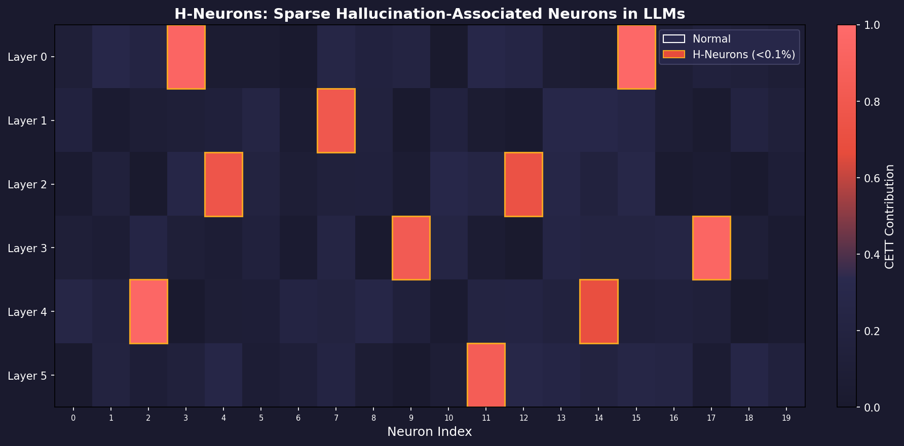
    return h_neuron_indices, weights

The result is striking: across six models (Mistral-7B, Mistral-Small-24B, Gemma-3-4B, Gemma-3-27B, Llama-3.1-8B, Llama-3.3-70B), the identified H-Neurons constitute less than 0.1% of total neurons, yet classifiers built on them achieve 70-84% accuracy on in-domain TriviaQA and generalize to out-of-distribution biomedical QA (BioASQ) and fabricated entity detection (NonExist).

Causal Intervention: Activation Scaling

To move from correlation to causation, the authors perturb H-Neurons at inference time by scaling their activations:

$$z_{j,t} \leftarrow \alpha \cdot z_{j,t}, \quad \alpha \in [0, 3]$$

where $\alpha < 1$ suppresses the neuron, $\alpha = 1$ is the baseline, and $\alpha > 1$ amplifies it. The authors show that under this perturbation, the CETT score scales approximately linearly:

$$\text{CETT}_{j,t}(\alpha) = \frac{\| \alpha \cdot h_t^{(j)} \|_2}{\| h_t + (\alpha - 1) h_t^{(j)} \|_2} \approx \alpha \cdot \text{CETT}_{j,t}$$

The approximation holds because any single neuron’s contribution $\| h_t^{(j)} \|_2$ is negligible relative to the full hidden state $\| h_t \|_2$ in models with thousands of neurons per layer.

def intervene_h_neurons(model, h_neuron_indices, alpha=0.0):
    """Register forward hooks to scale H-Neuron activations at inference."""
    
    hooks = []
    for layer in model.layers:
        def make_hook(layer_ffn):
            def hook_fn(module, input, output):
                # output is z_t after gate * up projection
                # Scale only the H-Neuron dimensions
                output[:, :, h_neuron_indices] *= alpha
                return output
            return hook_fn
        
        h = layer.ffn.activation_layer.register_forward_hook(
            make_hook(layer.ffn)
        )
        hooks.append(h)
    
    return hooks

def evaluate_with_intervention(model, tokenizer, prompts, h_neurons, alpha):
    hooks = intervene_h_neurons(model, h_neurons, alpha)
    
    results = []
    for prompt in prompts:
        inputs = tokenizer(prompt, return_tensors="pt")
        with torch.no_grad():
            output = model.generate(**inputs, max_new_tokens=256)
        results.append(tokenizer.decode(output[0], skip_special_tokens=True))
    
    for h in hooks:
        h.remove()
    
    return results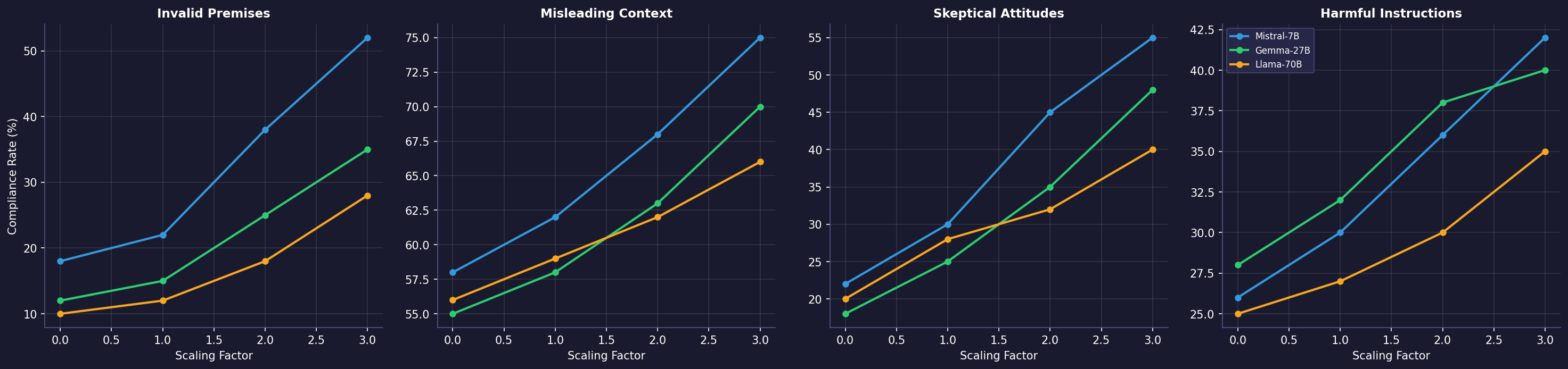

The results are the most interesting part of the paper. Amplifying H-Neurons ($\alpha > 1$) increases compliance rates across four distinct dimensions: accepting invalid premises (FalseQA), following misleading context (FaithEval), caving to skeptical pushback (Sycophancy), and complying with harmful instructions (Jailbreak). Suppressing them ($\alpha < 1$) reduces all four.

This suggests H-Neurons do not merely encode “factual incorrectness” but rather a general over-compliance disposition – the model’s tendency to satisfy the user at the expense of truthfulness, safety, or epistemic integrity.

Origin: Pre-training, Not Alignment

The final contribution traces H-Neurons back to pre-training. The authors apply classifiers trained on instruction-tuned models directly to their corresponding base models. AUROC scores remain well above chance (exceeding 86% on TriviaQA for the Mistral family), demonstrating that the neural signatures of hallucination exist before any RLHF or SFT.

To quantify how much alignment modifies these neurons, they compute the cosine distance between base and aligned model weights for each neuron’s up-projection and down-projection:

$$\Delta_j^{\text{up}} = 1 - \cos(W_{\text{up}}^{(j,\text{base})}, W_{\text{up}}^{(j,\text{chat})}), \quad \Delta_j^{\text{down}} = 1 - \cos(W_{\text{down}}^{(j,\text{base})}, W_{\text{down}}^{(j,\text{chat})})$$

These are z-scored and averaged. The finding: H-Neurons concentrate in the low-drift regime, meaning they are among the least modified neurons during alignment. Instruction tuning largely preserves these circuits rather than constructing them.

Critical Assessment

The paper makes a clean, well-structured argument, but several points deserve scrutiny:

1. The CETT metric measures magnitude, not direction. CETT captures $\| h_t^{(j)} \|_2 / \| h_t \|_2$ – the norm ratio. This tells us how much a neuron contributes but not in which direction in the residual stream. Two neurons with identical CETT scores could push the hidden state in opposite directions. A directional metric (e.g., the projection onto the unembedding direction of the correct vs. incorrect token) would be more informative for understanding the mechanism.

2. Linear probing is correlational by design. While the perturbation experiments do establish causation, the identification step remains correlational. The $\ell_1$ logistic regression identifies neurons whose activations correlate with hallucination, but this does not mean these neurons are the cause. They could be downstream read-outs of an earlier computational process. The causal graph is: perturbation changes behavior, but we cannot distinguish whether H-Neurons are drivers or mediators without more fine-grained ablation at different layers.

3. The over-compliance framing is compelling but unfalsifiable as stated. The paper reframes hallucination as a special case of over-compliance. This is a useful conceptual move, but the four benchmarks (FalseQA, FaithEval, Sycophancy, Jailbreak) all involve the model generating text in response to a prompt. Almost any behavioral change from neuron perturbation would show up as a “compliance” shift on at least some of these benchmarks. A stronger test would include a benchmark where suppressing H-Neurons should have no effect – a negative control.

4. The pre-training origin claim needs nuance. The backward transferability result is strong: classifiers transfer from chat to base models. But this proves that the pattern exists in base models, not that alignment doesn’t amplify it. The low-drift finding (H-Neurons are minimally modified by SFT) is more informative, but SFT with LoRA modifies very few parameters anyway – so most neurons show low drift regardless. The relevant comparison would be: is the drift of H-Neurons significantly lower than the average drift of neurons in the same layers?

5. Scalability of the identification pipeline. The method requires generating 10 responses per query (for consistency filtering), running GPT-4o for answer span extraction, computing CETT across all neurons and layers, and training a sparse classifier. For a 70B parameter model with thousands of neurons per layer across 80+ layers, this is a non-trivial computational pipeline that may not scale to rapid iteration.

6. Missing comparison with SAE-based approaches. Sparse autoencoders (Lindsey et al., 2025; Ferrando et al., 2025) decompose activations into interpretable features rather than raw neurons. The paper acknowledges this work but does not compare against it. SAE features are typically more monosemantic than individual neurons, so it is plausible that “hallucination features” identified via SAEs would be more interpretable and potentially fewer in number than H-Neurons.

Despite these caveats, the paper provides a valuable contribution: it demonstrates that hallucination is not a distributed, intractable phenomenon but is concentrated in an identifiable, sparse, and causally effective subset of the network’s computational units. This is encouraging for anyone working on interpretability-driven alignment.