The Lottery Ticket Hypothesis Jan 26, 2026

The Formal Statement

Let $f(x; \theta)$ be a dense neural network with initial parameters $\theta_0 \sim \mathcal{D}_\theta$. Training this network for $T$ iterations with SGD yields parameters $\theta_T$ that achieve test accuracy $a$ in validation time $t$.

The Lottery Ticket Hypothesis states:

There exists a binary mask $m \in \{0, 1\}^{|\theta|}$ such that the sparse subnetwork $f(x; m \odot \theta_0)$, when trained for at most $T'$ iterations, achieves test accuracy $a' \geq a$ in validation time $t' \leq t$, where $\|m\|_0 \ll |\theta|$.

Here $\odot$ denotes element-wise multiplication (Hadamard product), and $\|m\|_0$ is the number of non-zero entries in the mask. The key insight: the initial weights $\theta_0$ matter. The same mask with a different random initialization does not produce a winning ticket.

Iterative Magnitude Pruning (IMP)

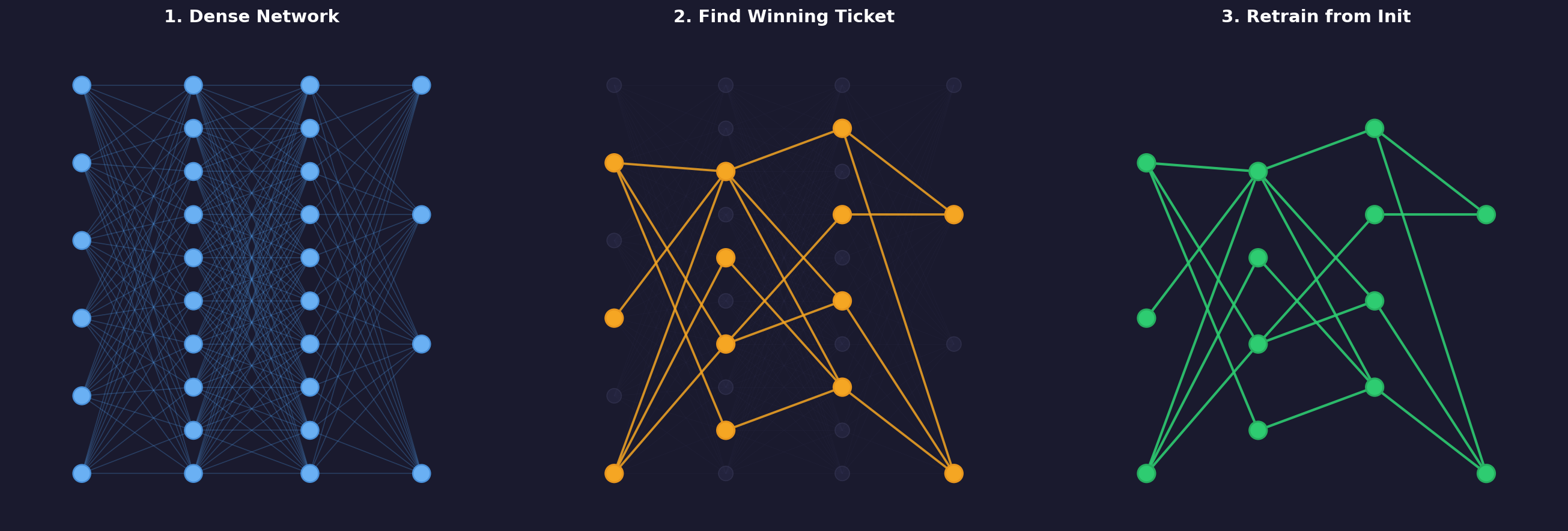
The authors propose Iterative Magnitude Pruning as the algorithm to find winning tickets. The idea is simple: train the network, remove the smallest weights, then reset the surviving weights to their original initialization and retrain.

Given a pruning rate $p$ per round and $n$ rounds of pruning, the final sparsity after $n$ rounds is:

$$s = 1 - (1 - p)^n$$

For example, with $p = 0.2$ (prune 20% each round) and $n = 10$ rounds, the final sparsity is $s = 1 - 0.8^{10} \approx 89.3\%$, meaning nearly 90% of the weights are removed.

The pruning criterion at each round selects weights by magnitude:

$$m_j = \begin{cases} 1 & \text{if } |\theta_j^{(T)}| > \tau_p \\ 0 & \text{otherwise} \end{cases}$$

where $\tau_p$ is the $p$-th percentile of the absolute weight values of the surviving weights.

Pseudocode

def iterative_magnitude_pruning(model, train_data, prune_rate, num_rounds):
    # Step 1: Save the original random initialization
    theta_0 = copy(model.parameters())
    
    # Start with all weights active
    mask = ones_like(theta_0)
    
    for round in range(num_rounds):
        # Step 2: Reset surviving weights to their original initialization
        model.parameters = theta_0 * mask
        
        # Step 3: Train the masked network to completion
        for epoch in range(num_epochs):
            for batch in train_data:
                output = model.forward(batch.x, mask)
                loss = cross_entropy(output, batch.y)
                gradients = backward(loss)
                # Only update weights that are not pruned
                model.parameters -= learning_rate * gradients * mask
        
        # Step 4: Prune the smallest weights by magnitude
        surviving_weights = abs(model.parameters[mask == 1])
        threshold = percentile(surviving_weights, prune_rate * 100)
        
        # Zero out weights below the threshold
        new_mask = (abs(model.parameters) >= threshold).float()
        mask = mask * new_mask
        
        sparsity = 1.0 - sum(mask) / len(mask)
        accuracy = evaluate(model, test_data, mask)
        print(f"Round {round}: sparsity={sparsity:.1%}, accuracy={accuracy:.2f}")
    
    return mask, theta_0

Why Initialization Matters

The most surprising finding is that the initial weights are critical. Consider three experiments at the same sparsity level:

1. Winning Ticket (same mask + original init $\theta_0$): Matches or exceeds full network accuracy
2. Same mask + random reinit $\theta_0'$: Performance degrades significantly
3. Random mask + original init: Poor performance

This can be understood through the lens of the loss landscape. The initialization $\theta_0$ places the subnetwork in a favorable basin of attraction. The mask $m$ selects exactly those weights that, from this starting point, can navigate to a good minimum:

$$\mathcal{L}(m \odot \theta_0) \xrightarrow{\text{SGD}} \theta^* \quad \text{(low loss minimum)}$$

$$\mathcal{L}(m \odot \theta_0') \xrightarrow{\text{SGD}} \theta^{*'} \quad \text{(higher loss minimum)}$$

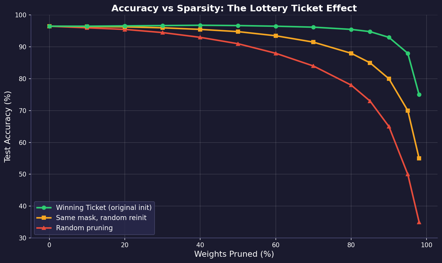
The chart above illustrates this effect. The winning ticket (green) maintains high accuracy even at extreme sparsity levels (80-90% of weights removed). The same pruning mask with a random reinitialization (orange) degrades earlier, and random pruning (red) collapses quickly. This confirms the hypothesis: it is the combination of structure (mask) and initialization that makes a winning ticket.

Connection to Magnitude Pruning Theory

Why does magnitude-based pruning work? One way to think about it is through the Taylor expansion of the loss function. When we remove weight $\theta_j$ (set it to zero), the change in loss is approximately:

$$\Delta \mathcal{L}_j \approx -g_j \theta_j + \frac{1}{2} h_j \theta_j^2$$

where $g_j = \frac{\partial \mathcal{L}}{\partial \theta_j}$ is the gradient and $h_j = \frac{\partial^2 \mathcal{L}}{\partial \theta_j^2}$ is the Hessian diagonal. At a converged minimum, $g_j \approx 0$, so:

$$\Delta \mathcal{L}_j \approx \frac{1}{2} h_j \theta_j^2$$

If we further assume $h_j$ is roughly constant across weights (a crude but useful approximation), then $\Delta \mathcal{L}_j \propto \theta_j^2$. This justifies pruning the smallest-magnitude weights: they cause the least damage when removed.

More sophisticated methods like Optimal Brain Surgeon use the full Hessian $\mathbf{H}$ to compute the optimal weight to remove:

$$\text{saliency}_j = \frac{\theta_j^2}{2 [H^{-1}]_{jj}}$$

but magnitude pruning remains the practical workhorse due to its simplicity.

A Complete Experiment

Here is a complete implementation of the Lottery Ticket Hypothesis experiment on MNIST with a simple feedforward network:

import torch
import torch.nn as nn
import torch.optim as optim
from torchvision import datasets, transforms
from copy import deepcopy

class SimpleNet(nn.Module):
    def __init__(self):
        super().__init__()
        self.fc1 = nn.Linear(784, 300)
        self.fc2 = nn.Linear(300, 100)
        self.fc3 = nn.Linear(100, 10)
    
    def forward(self, x, masks=None):
        x = x.view(-1, 784)
        if masks:
            x = torch.relu(self.fc1(x) * masks[0])
            x = torch.relu(self.fc2(x) * masks[1])
            x = self.fc3(x) * masks[2]
        else:
            x = torch.relu(self.fc1(x))
            x = torch.relu(self.fc2(x))
            x = self.fc3(x)
        return x

def train(model, loader, masks, epochs=10, lr=0.01):
    optimizer = optim.SGD(model.parameters(), lr=lr)
    criterion = nn.CrossEntropyLoss()
    for epoch in range(epochs):
        for data, target in loader:
            optimizer.zero_grad()
            output = model(data, masks)
            loss = criterion(output, target)
            loss.backward()
            # Zero gradients for pruned weights
            if masks:
                for param, mask in zip(model.parameters(), masks):
                    if param.grad is not None:
                        param.grad *= mask
            optimizer.step()

def evaluate(model, loader, masks=None):
    correct = 0
    total = 0
    with torch.no_grad():
        for data, target in loader:
            output = model(data, masks)
            pred = output.argmax(dim=1)
            correct += (pred == target).sum().item()
            total += target.size(0)
    return correct / total

def prune_by_magnitude(model, masks, prune_rate):
    new_masks = []
    for param, mask in zip(model.parameters(), masks):
        alive = param.data.abs()[mask == 1]
        threshold = torch.quantile(alive, prune_rate)
        new_mask = ((param.data.abs() >= threshold) * mask).float()
        new_masks.append(new_mask)
    return new_masks

def lottery_ticket_experiment(prune_rate=0.2, rounds=5):
    train_loader = torch.utils.data.DataLoader(
        datasets.MNIST('.', train=True, download=True,
                       transform=transforms.ToTensor()),
        batch_size=128, shuffle=True)
    test_loader = torch.utils.data.DataLoader(
        datasets.MNIST('.', train=False,
                       transform=transforms.ToTensor()),
        batch_size=512)
    
    # Initialize model and save original weights
    model = SimpleNet()
    initial_state = deepcopy(model.state_dict())
    
    # Initialize masks (all ones = no pruning)
    masks = [torch.ones_like(p) for p in model.parameters()]
    
    for r in range(rounds):
        # Reset to original initialization with current mask
        model.load_state_dict(initial_state)
        for param, mask in zip(model.parameters(), masks):
            param.data *= mask
        
        # Train
        train(model, train_loader, masks)
        accuracy = evaluate(model, test_loader, masks)
        
        # Compute sparsity
        total = sum(m.numel() for m in masks)
        alive = sum(m.sum().item() for m in masks)
        sparsity = 1 - alive / total
        
        print(f"Round {r}: sparsity={sparsity:.1%}, acc={accuracy:.4f}")
        
        # Prune
        masks = prune_by_magnitude(model, masks, prune_rate)
    
    return masks, initial_state

lottery_ticket_experiment()

Late Rewinding

In follow-up work https://arxiv.org/abs/1903.01611, Frankle et al. found that for deeper networks (ResNets, VGGs), resetting to the exact initialization $\theta_0$ no longer works reliably. Instead, they propose late rewinding: resetting to weights at iteration $k$ early in training, rather than iteration 0:

$$\theta_{\text{rewind}} = \theta_k \quad \text{where } k \ll T$$

Typically $k$ corresponds to 1-5% of total training. This small amount of initial training moves the weights into a better region of the loss landscape, after which the mask becomes effective. This variant is sometimes called the Stabilized Lottery Ticket Hypothesis and has been shown to scale to ImageNet-level tasks.

Connections to Other Sparsity Methods

The Lottery Ticket Hypothesis connects deeply to other sparsity research:

• Mixture of Experts (MoE): MoE achieves conditional sparsity at inference time by routing tokens to a subset of experts. The lottery ticket perspective suggests that MoE might work because each expert is, in a sense, a winning ticket for its input distribution. The routing network learns to match inputs to their best subnetwork.

• Sparse Autoencoders (SAE): SAEs enforce sparsity in activations, meaning few neurons fire for any given input. Lottery tickets enforce sparsity in weights, meaning few connections exist at all. Both converge on the idea that neural networks are vastly over-parameterized and that most computation is redundant.

• Quantization: Quantization reduces the bits per weight, while pruning reduces the number of weights. They are complementary: a winning ticket can be further quantized. Recent work on SparseGPT combines unstructured pruning with quantization to achieve 60% sparsity + 4-bit weights with minimal accuracy loss on LLMs.

• Neural Collapse: At the end of training, features collapse to class means forming a simplex ETF. The lottery ticket hypothesis suggests that only a subset of the network is responsible for learning these collapsed representations, raising the question: do winning tickets exhibit neural collapse faster?

Open Questions

Several important questions remain:

1. Is there a theory of winning tickets? We know they exist empirically, but we lack a theory predicting which initializations will contain good tickets.

2. Can we find tickets without training? Methods like SNIP (Single-shot Network Pruning) and GraSP attempt to identify sparse masks at initialization, before any training occurs.

3. Do LLMs have lottery tickets? Recent work suggests yes, and that different tasks may activate different subnetworks within a large model, echoing the MoE philosophy.

4. Strong vs. Weak tickets: Some tickets not only match but exceed the dense network’s performance. Understanding when and why this happens remains open.