Kolmogorov-Arnold Networks Sep 21, 2024

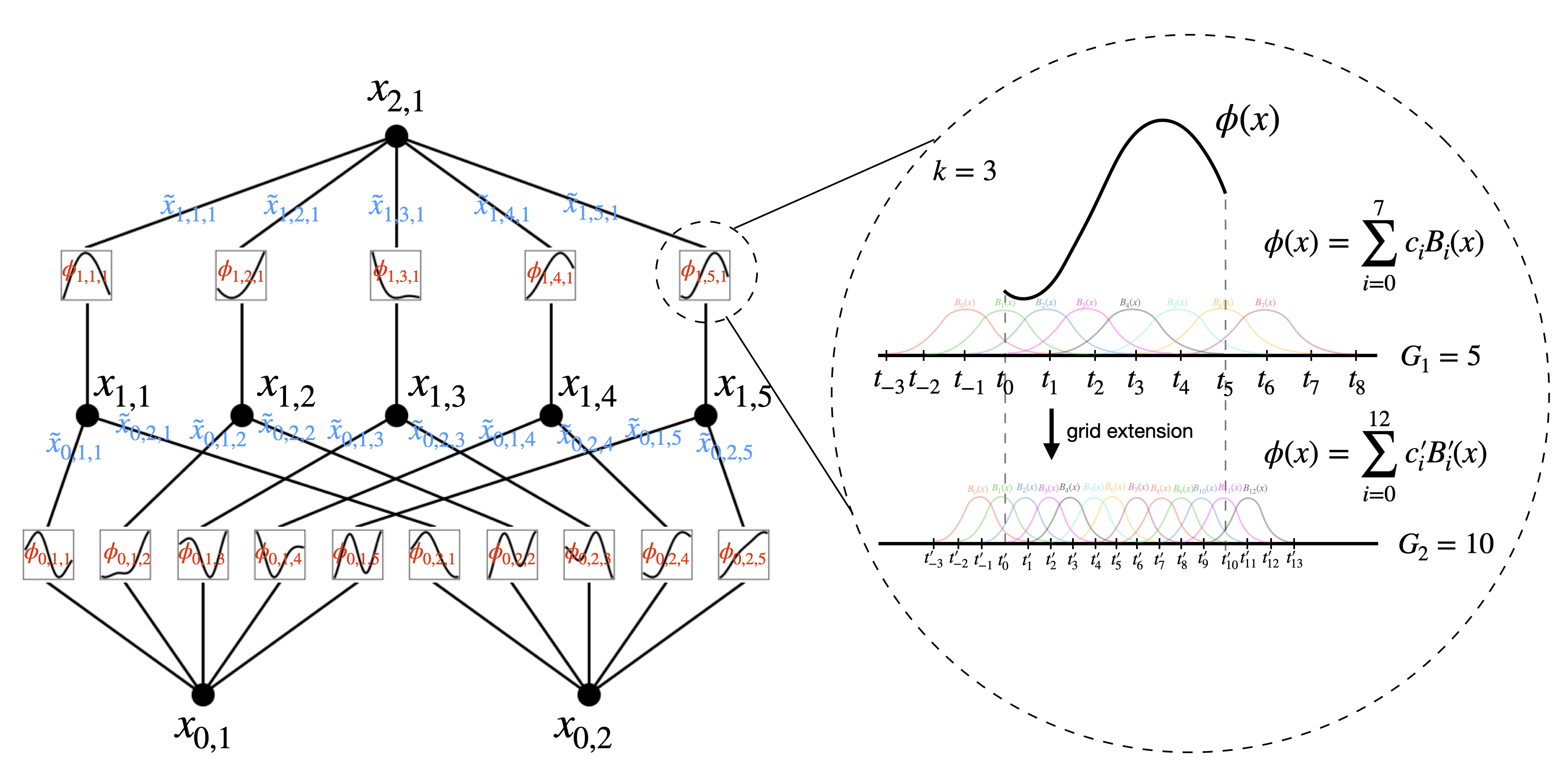
I have been playing with some implementations of Kolmogorov-Arnold Networks. Here is an easy implementation for anyone who wants to try it out.

In general, the promising ideas showed on the original paper are not so easy to replicate. I personally believe that KAN’s are a promising research direction, but maybe the hype on the original paper created an unrealistic expectation on the capabilities of KAN’s for now.

For more details here is the colab where I implemented the models Link to code