DDIM vs DDPM Sep 9, 2024

DDPM

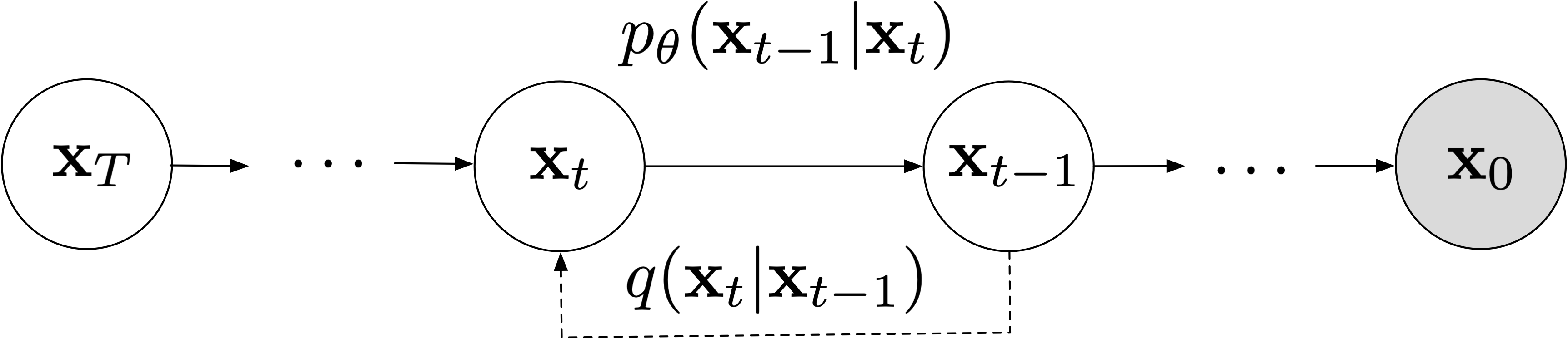
DDPM, introduced by Ho et al. in their 2020 paper “Denoising Diffusion Probabilistic Models,” is grounded in the principles of non-equilibrium thermodynamics. The model defines a Markov chain of diffusion steps that gradually add Gaussian noise to data, and then learns to reverse this process. Here’s a simplified pseudocode representation of the DDPM sampling process:

def sample_ddpm(num_steps):
    x = random_noise()
    for t in reversed(range(num_steps)):
        z = random_noise() if t > 1 else 0
        noise_pred = denoise_fn(x, t)
        x = (1 / sqrt(1 - beta[t])) * (x - (beta[t] / sqrt(1 - alpha_bar[t])) * noise_pred) + sqrt(beta[t]) * z
    return x

In this pseudocode, beta represents the noise schedule, alpha_bar is the cumulative product of (1 - beta), and denoise_fn is the learned denoising function.

DDPM is characterized by its Markovian nature, where each step depends only on the immediately preceding step. It typically employs a fixed number of steps, usually around 1000, for the denoising process. The generation process in DDPM involves stochastic sampling, drawing from probability distributions at each step. This approach generally yields high-quality samples but at the cost of computational intensity due to the large number of steps involved.

DDIM

DDIM, proposed by Song et al. in their 2020 paper “Denoising Diffusion Implicit Models,” builds upon DDPM while introducing significant modifications to the generative process. DDIM introduces a non-Markovian inference process. Here’s a simplified pseudocode representation of the DDIM sampling process:

def sample_ddim(num_steps, eta):
    x = random_noise()
    for t in reversed(range(num_steps)):
        noise_pred = denoise_fn(x, t)
        alpha = alpha_bar[t]
        alpha_next = alpha_bar[t-1] if t > 0 else 1.0
        sigma = eta * sqrt((1 - alpha / alpha_next) * (1 - alpha_next) / (1 - alpha))
        z = random_noise() if t > 1 else 0
        x = sqrt(alpha_next) * (x - sqrt(1 - alpha) * noise_pred) / sqrt(alpha)
        x = x + sqrt(1 - alpha_next - sigma**2) * noise_pred + sigma * z
    return x

In this pseudocode, eta is a hyperparameter controlling the stochasticity of the sampling process. When eta = 0, the process becomes deterministic.

The key advancements in DDIM include its non-Markovian process, where each step can depend on multiple previous steps, and the option for deterministic sampling by setting eta to 0. Perhaps most notably, DDIM allows for flexible sampling steps, capable of generating samples using significantly fewer steps (e.g., 10-100) compared to DDPM.

When comparing the two models, several key differences emerge. In terms of sampling efficiency, DDPM requires a fixed number of steps, resulting in slower generation. DDIM, on the other hand, allows for accelerated sampling with fewer steps, significantly reducing generation time. This efficiency gain in DDIM comes with a potential trade-off in sample quality, especially at very low step counts, though it can generally maintain comparable quality to DDPM.

The latent space properties of these models also differ significantly. DDPM’s stochastic nature makes it challenging to manipulate the latent space directly. In contrast, DDIM’s deterministic option allows for more controlled latent space manipulation, enabling operations like interpolation.

From a theoretical standpoint, DDPM provides stronger guarantees due to its well-defined probabilistic framework. DDIM, while sacrificing some theoretical rigor, gains practical advantages in sampling speed and control. Both models can utilize similar neural network architectures, such as U-Net, for the denoising function. Notably, DDIM requires minimal modifications to a pre-trained DDPM model, making it an attractive upgrade option.