foundational-brain 2026
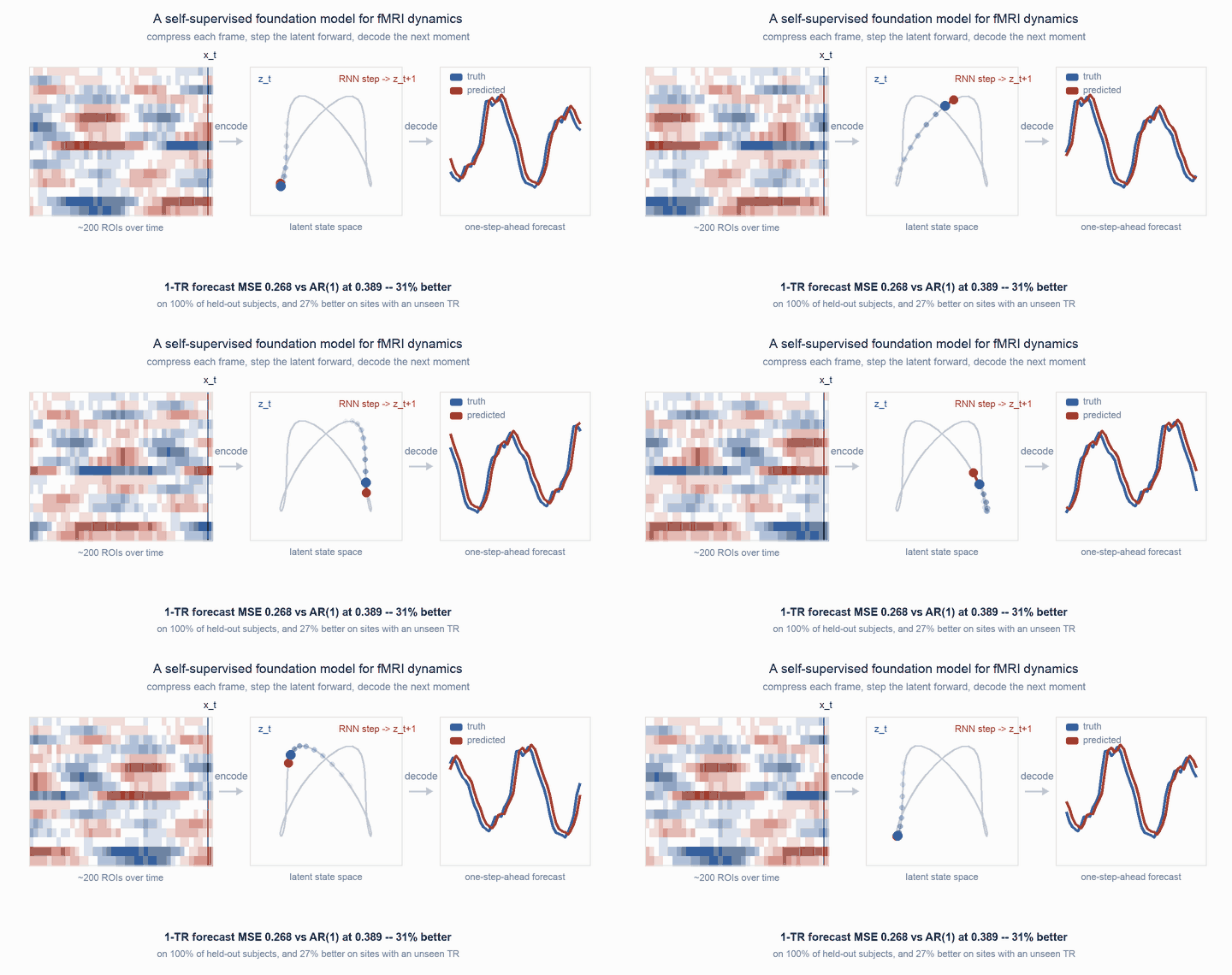
What does a foundation model for the brain actually learn? This project builds one from three composable parts — an encoder that compresses a single fMRI frame into a latent vector, a recurrent core that models how those latents evolve, and a decoder that maps them back to brain space — and then takes the answer seriously, including where it is unflattering.
No labels, no downstream task baked in. The model is trained purely to predict the next moment of brain activity.
The setup #
fMRI is a 4-D signal (X, Y, Z, T). Each volume is projected onto a brain atlas
to give a T × N_regions matrix of ROI time series — the standard,
scanner-comparable representation. The corpus is ABIDE-PCP: 871
quality-checked resting-state subjects across 20 sites, already parcellated,
fully open.
The three self-supervised objectives are trained jointly:
-
Reconstruction —
‖D(E(x_t)) − x_t‖², which keeps the latent informative. -
Latent forecasting —
‖F(z_{1:t}) − z_{t+1}‖², the core dynamics objective. - Masked latent modeling — mask timepoints, reconstruct them from context.
Letting the data set the hyperparameters #
Profiling all 871 subjects before training changed the plan in ways worth recording:
-
A brain frame is not low-rank. 125 of 200 components are needed for 90% of
frame variance. The originally configured
latent_dim=256exceeded the input dimension — an expansion, not a bottleneck. Now 128. - Forecasting only works at one step. At a 2-TR horizon both persistence and AR(1) are already worse than predicting the mean, so a multi-step objective would be fitting noise.
- Sites do not share a repetition time. Lag-1 autocorrelation ranges 0.534 to 0.874 across sites — “one step” means a different amount of elapsed time depending on where the subject was scanned. Resolved by partition: pretrain on the TR = 2.0 s group (10 sites, 522 subjects) and hold the rest out as a cross-TR test.
-
But the dynamics are not AR(1) either.
acf(2)/acf(1)²sits at 0.43–0.72 where a first-order Markov process would give exactly 1.0 — so a model with memory has genuine headroom.
What worked #
The dynamics half delivers. Against an AR(1) bar of 0.389, the latent RNN reaches 0.268 validation 1-TR forecast MSE — 31% better — and it is better on 100% of held-out subjects on both splits (Wilcoxon p = 3.5e-10, so this is not an outlier-carried average). On 349 subjects from sites whose repetition time was never seen during training it still wins by 27%, so the representation is not just memorizing one sampling rate.
What didn’t, and why that’s the interesting part #
- The spatial map is essentially linear. The encoder never beats PCA at a matched width — at every width from 8 to 128, with the gap growing from 0.7% to 10%. The nonlinear encoder earns nothing for pure reconstruction. The useful consequence is a clean decomposition: the model’s entire advantage over baselines lives in the temporal core.
-
Reconstruction is an ally, not a competitor. I expected down-weighting
reconstruction to free the latent for forecasting. The opposite held: forecast
MSE is best at
w_reconstruction = 1.0and degrades as it is down-weighted. The default 1:1:1 was validated rather than changed. - Pooling mattered more than the representation. Under mean+std pooling, phenotype decoding looked weak (DX AUC ≈ 0.63). Under connectivity pooling — where resting-state phenotype signal actually lives — it jumps to DX 0.76, sex 0.78, age R² 0.43. The weak first result was largely a pooling artifact.
-
The model does not beat raw functional connectivity. For diagnosis and sex,
raw_fcmatches or beats the learned features; only age shows a model win. And the RNN’s features stay the most site-decodable of all (0.835).
So: the model forecasts well and encodes real temporal structure, but those dynamics are not yet a clean, biology-carrying transfer representation — they are partly acquisition. It learned the scanner as much as the brain. That result is what makes the next step obvious: site-adversarial pretraining, with the test being whether site-decodability falls while forecasting and phenotype hold.
What’s inside #
Python 3.12 with PyTorch and nilearn, managed by uv; 58 tests; ~7 minutes to
pretrain 60 epochs on an M-series GPU. Every claim above is backed by a generated
report in docs/ — the corpus profile, the latent-width sweep, the loss-weight
sweep, and both probe analyses.
There is also a visual explainer: an animated, layman-friendly walkthrough of what the model predicts and what it did and didn’t learn, with every animation driven by real ABIDE scans and the trained model rather than mock-ups.