Mixture of Experts Aug 4, 2025

In the pursuit of scaling neural networks to unprecedented parameter counts while maintaining computational tractability, the paradigm of conditional computation has emerged as a cornerstone of modern deep learning architectures. A prominent and highly successful incarnation of this principle is the Mixture of Experts (MoE) layer. At its core, an MoE model eschews the monolithic, dense activation of traditional networks, wherein every parameter is engaged for every input. Instead, it employs a collection of specialized subnetworks, termed “experts,” and dynamically selects a sparse combination of these experts to process each input token. This approach allows for a dramatic increase in model capacity without a commensurate rise in computational cost (FLOPs), as only a fraction of the network’s parameters are utilized for any given forward pass.

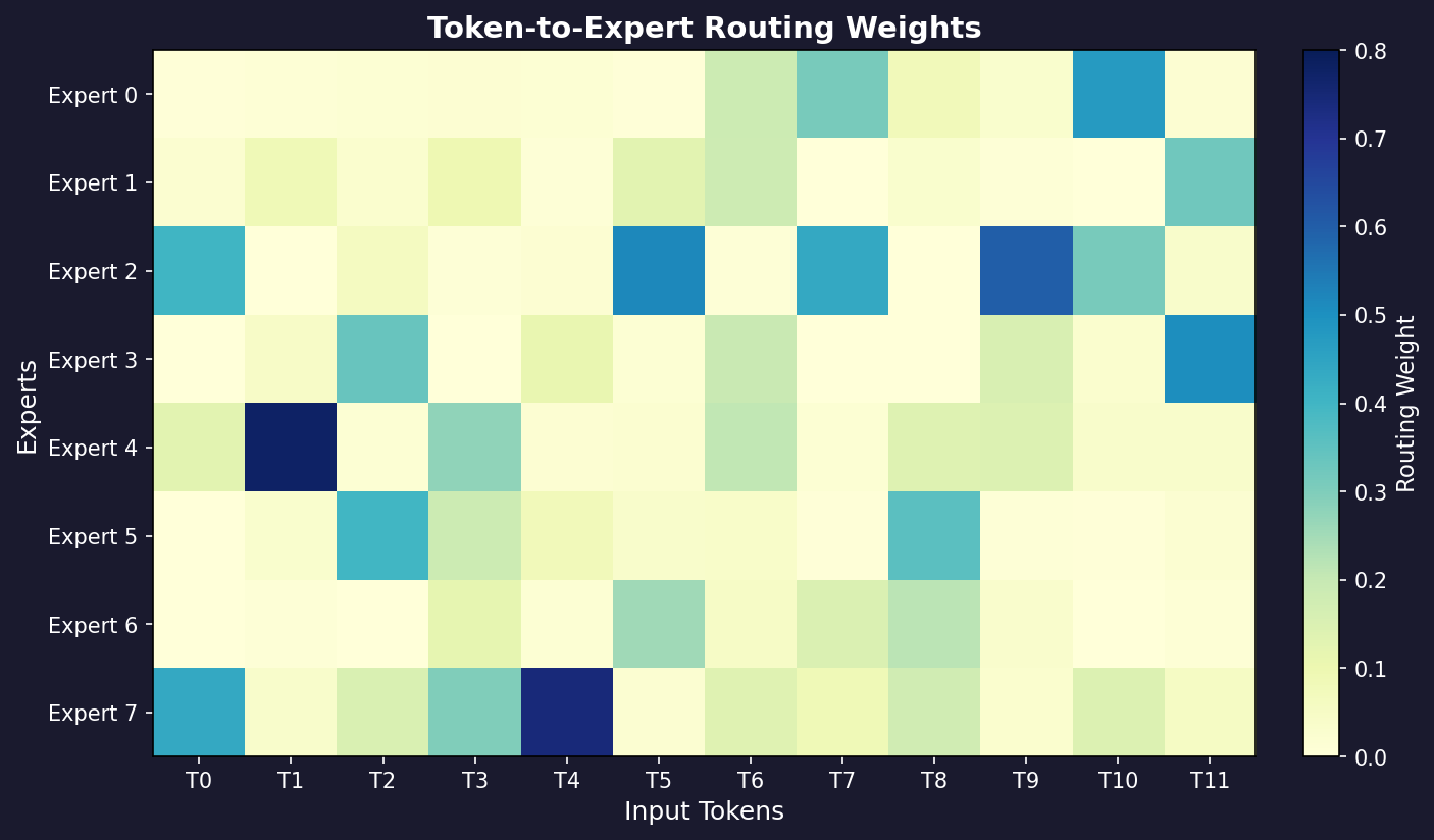
The architecture is orchestrated by two primary components: a set of N expert networks, E1, E2, …, E_N, and a trainable gating network, G. The expert networks are typically homogenous in their architecture (e.g., small feed-forward networks) but learn distinct functions over the course of training. The gating network, often a simple linear layer followed by a softmax function, serves as a dynamic router. For a given input vector x, the gating network produces a normalized distribution of weights over the N experts, effectively learning to predict which experts are most suitable for processing that specific input.

The final output of the MoE layer, y, is not the output of a single chosen expert but rather a weighted sum of the outputs from all experts. The weights for this summation are precisely the probabilities generated by the gating network. The output is thus computed as: y = \sum^{N} gi(x) E_i(x) where E_i(x) is the output of the i-th expert for the input x, and g(x) is the vector of gating weights produced by the gating network G. The weights are typically computed via a softmax over the logits.

In practice, to enforce sparsity and reduce computation, a variant known as the Sparse Mixture of Experts is commonly deployed. In this formulation, only the experts with the highest gating weights—the “top-k” experts, where $k$ is a small integer (e.g., 1 or 2)—are activated. The gating weights are re-normalized over this small subset of selected experts. This ensures that the computational cost is independent of the total number of experts, N, and dependent only on k. This sparse, conditional activation is the key to the MoE’s efficiency.

# Let x be the input token representation
# Let E be the set of N expert networks {E_1, ..., E_N}
# Let G be the gating network
# Let k be the number of experts to select

# 1. Compute gating logits for the input token x.
# W_g is the weight matrix of the gating network.
logits = G(x)  # Shape: [N]

# 2. Select the top k experts.
# Get the k largest logit values and their corresponding indices.
top_k_logits, top_k_indices = TopK(logits, k)

# 3. Compute the normalized routing weights for the selected experts.
# Apply softmax only to the selected logits to get sparse weights.
routing_weights = Softmax(top_k_logits) # Shape: [k]

# 4. Initialize the final output vector.
# The output has the same dimension as the expert outputs.
final_output = 0

# 5. Compute the weighted sum of the selected expert outputs.
# Iterate through the chosen experts and their corresponding weights.
for i in 1..k:
    # Get the index of the i-th expert in the top-k set.
    expert_index = top_k_indices[i]

    # Get the routing weight for this expert.
    weight = routing_weights[i]

    # Retrieve the corresponding expert network.
    selected_expert = E[expert_index]

    # Process the input token with the selected expert.
    expert_output = selected_expert(x)

    # Accumulate the weighted expert output.
    final_output += weight * expert_output

# 6. Return the combined output.
# This output is then passed to the next layer in the network.
return final_output