Deepseek, an overview and quick notes
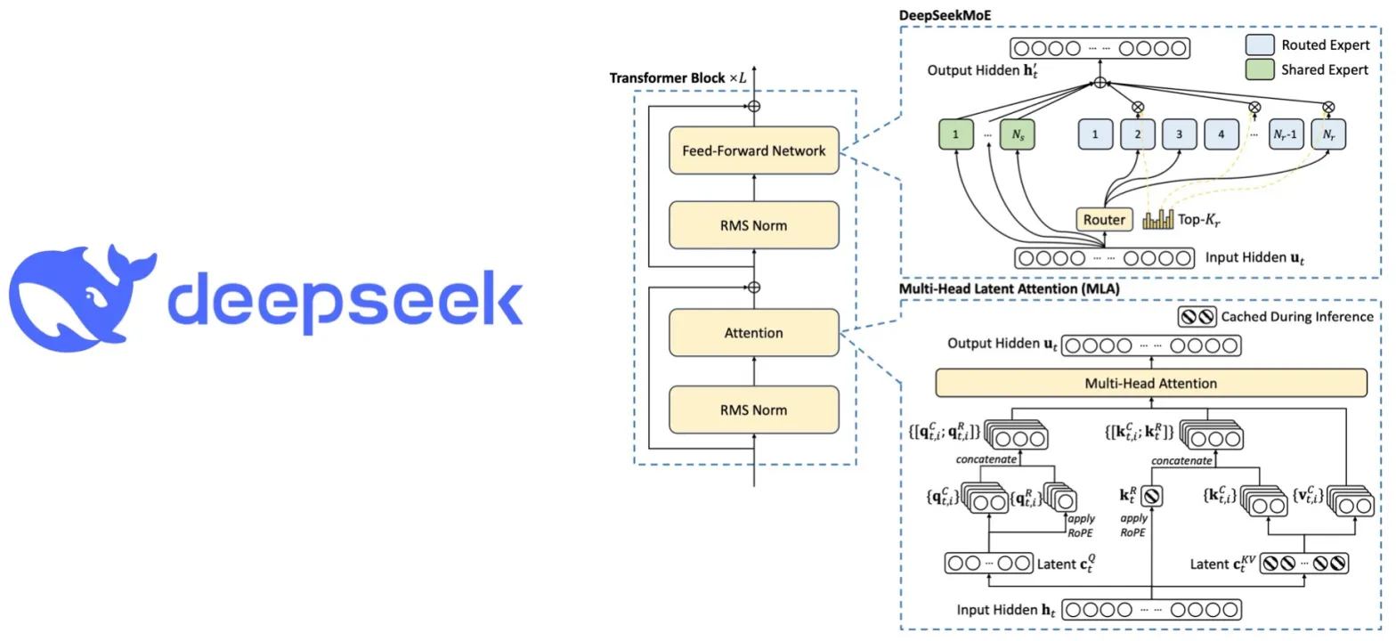
When DeepSeek-V3 came out I first wrote these notes as a bullet list of its headline claims. The numbers are striking, but what interested me more were the architectural tricks that make a 671B-parameter model cheap to train and cheap to serve. So I went back to the technical report and worked through the main ideas properly: how Multi-head Latent Attention shrinks the KV cache, how the MoE layers are routed, the auxiliary-loss-free load balancing rule (with a small simulation you can play with), multi-token prediction, and a short note on the FP8 and pipeline-parallel engineering.
Key numbers #
- Size: a Mixture-of-Experts model with 671B total parameters, of which 37B are activated per token. It has 61 layers with hidden size 7168.
- Data: pre-trained on 14.8T tokens with a 4K context. The context was then extended in two stages (4K → 32K → 128K) with YaRN, 1000 steps each.
- Compute: 2.788M H800 GPU hours in total: 2664K for pre-training, 119K for context extension and 5K for post-training. At an assumed rental price of 2 USD per GPU hour this comes to 5.576M USD. That figure covers only the final training run. The report says explicitly that it excludes prior research and ablation experiments.
- Benchmarks (chat model): 90.2 on MATH-500, the 51.6th percentile on Codeforces, and 75.9 on MMLU-Pro.
- Against closed models: the report compares against GPT-4o (0513) and Claude-3.5-Sonnet (1022). V3 beats both on MATH-500 (74.6 and 78.3) and Codeforces (23.6 and 20.3). On MMLU-Pro it beats GPT-4o (72.6) but trails Claude (78.0). So “competitive” is the fair word, not “better across the board”.
Multi-head Latent Attention (MLA) #
At inference time, autoregressive decoding is dominated by the KV cache. For every past token and every layer you keep its keys and values so you do not have to recompute them. Standard multi-head attention (MHA) with $n_h$ heads of dimension $d_h$ caches $2 n_h d_h$ numbers per token per layer. Grouped-query attention (GQA) shares each K/V head across a group of query heads and caches $2 n_g d_h$ numbers. Multi-query attention (MQA) goes all the way down to $2 d_h$. Both shrink the cache by throwing away K/V capacity.
MLA, introduced in DeepSeek-V2 and reused in V3, takes a different route: low-rank joint compression of keys and values. For the attention input $h_t \in \mathbb{R}^d$ of token $t$, it computes a single small latent vector
$$c_t^{KV} = W^{DKV} h_t, \qquad c_t^{KV} \in \mathbb{R}^{d_c},\; d_c \ll n_h d_h$$
and reconstructs the per-head keys and values from it with up-projections:
$$k_t^{C} = [k_{t,1}^C; \dots; k_{t,n_h}^C] = W^{UK} c_t^{KV}, \qquad v_t^{C} = [v_{t,1}^C; \dots; v_{t,n_h}^C] = W^{UV} c_t^{KV}$$
with $W^{UK}, W^{UV} \in \mathbb{R}^{n_h d_h \times d_c}$. Only $c_t^{KV}$ needs to be cached. The queries are compressed the same way, $c_t^Q = W^{DQ} h_t$ with $d_c' = 1536$ and $q_t^C = W^{UQ} c_t^Q$. That does nothing for the cache but saves activation memory during training.
Why the up-projections disappear at inference #
The trick that makes this cheap is that you never actually materialise $k^C$ and $v^C$. For head $i$ the attention logit is
$${q_{t,i}^C}^\top k_{j,i}^C = \big(W^{UQ}_i c_t^Q\big)^\top W^{UK}_i c_j^{KV} = {c_t^Q}^\top \underbrace{\big({W^{UQ}_i}^\top W^{UK}_i\big)}_{\text{precompute once}} c_j^{KV}$$
so $W^{UK}$ can be absorbed into the query projection, and the query attends directly over the cached latents. Likewise $W^{UV}$ can be folded into the output projection $W^O$, because $\sum_j a_{tj} W^{UV}_i c_j^{KV} = W^{UV}_i \sum_j a_{tj} c_j^{KV}$.
The decoupled RoPE key #
Rotary position embeddings break this. RoPE multiplies queries and keys by position-dependent rotations $R_t$ and $R_j$, so the logit becomes
$$\big(R_t W^{UQ}_i c_t^Q\big)^\top R_j W^{UK}_i c_j^{KV} = {c_t^Q}^\top {W^{UQ}_i}^\top R_{j-t}\, W^{UK}_i\, c_j^{KV}.$$
Now there is a rotation, which depends on the relative position $j - t$, stuck between the two matrices. There is no single matrix to precompute. You would have to rebuild the full keys for every cached token at every step, which defeats the purpose.
DeepSeek’s fix is to decouple position from content. Each head’s key gets a few extra dimensions that carry RoPE, computed directly from $h_t$ and shared across all heads:
$$k_t^R = \operatorname{RoPE}\big(W^{KR} h_t\big) \in \mathbb{R}^{d_h^R}, \qquad k_{t,i} = [k_{t,i}^C;\, k_t^R]$$
The matching query part $q_{t,i}^R = \operatorname{RoPE}(W^{QR} c_t^Q)$ is per head. The attention output for head $i$ is
$$o_{t,i} = \sum_{j \le t} \operatorname{Softmax}_j\!\left( \frac{q_{t,i}^\top k_{j,i}}{\sqrt{d_h + d_h^R}}\right) v_{j,i}^C , \qquad u_t = W^O [o_{t,1}; \dots; o_{t,n_h}].$$
The content part still goes through the absorbed latent path. Only the small RoPE part uses explicit positions. What gets cached per token per layer is therefore $c_t^{KV}$ and $k_t^R$, which is $d_c + d_h^R$ numbers. (This shared $k_t^R$ is also the part YaRN is applied to during context extension.)
KV cache per token #
| Mechanism | Cached elements per token per layer |
|---|---|
| MHA | $2 n_h d_h$ |
| GQA ($n_g$ groups) | $2 n_g d_h$ |
| MQA | $2 d_h$ |
| MLA | $d_c + d_h^R$ |
With V3’s real dimensions, $n_h = 128$, $d_h = 128$, $d_c = 512$ (that is $4 d_h$), and $d_h^R = 64$ (that is $d_h / 2$):
- MHA: $2 \times 128 \times 128 = 32{,}768$ elements.
- MLA: $512 + 64 = 576$ elements.
That is a ratio of $32768 / 576 \approx 56.9\times$ against an MHA model with the same heads. In GQA terms, $576 = 2 \times 2.25 \times 128$, so MLA caches as much as GQA with only 2.25 groups. The DeepSeek-V2 paper makes the same comparison and claims MLA still performs better than MHA. Over all 61 layers in BF16 this is about 68.6 KiB per token, against 3.8 MiB for MHA.
The block below works the comparison out for a full 128K context (“elems” is per token per layer). Press Run (it uses Pyodide with NumPy, so the first run takes a few seconds).
import numpy as np

# DeepSeek-V3 attention dimensions (Section 4.2 of the technical report)
n_layers = 61
n_heads  = 128     # n_h
d_head   = 128     # d_h
d_c      = 512     # KV compression dim
d_rope   = 64      # decoupled RoPE key dim, d_h^R
bytes_per = 2      # BF16 cache
context  = 128 * 1024

# Elements cached per token, per layer
schemes = {
    "MHA (128 KV heads)": 2 * n_heads * d_head,
    "GQA (8 KV groups)":  2 * 8 * d_head,
    "MQA (1 KV head)":    2 * 1 * d_head,
    "MLA (d_c + d_h^R)":  d_c + d_rope,
}

elems = np.array(list(schemes.values()), dtype=np.int64)
per_token_bytes = elems * n_layers * bytes_per
total_gib = per_token_bytes * context / 2**30

print(f"context = {context:,} tokens, {n_layers} layers, BF16\n")
print(f"{'scheme':<20}{'elems':>7}{'KiB/tok':>9}{'GiB@128K':>10}{'vs MLA':>8}")
mla = elems[-1]
for name, e, b, g in zip(schemes, elems, per_token_bytes, total_gib):
    print(f"{name:<20}{e:>7,}{b / 1024:>9.1f}{g:>10.2f}{e / mla:>7.2f}x")

print(f"\nMLA caches the same as GQA with {mla / (2 * d_head):.2f} groups")A single 128K sequence needs about 8.6 GiB of cache with MLA, against roughly 488 GiB with full MHA at the same width. That is most of the 640 GB of HBM on an 8×H800 node, spent on the cache of a single sequence.
DeepSeekMoE #
Every FFN except those in the first three layers is a DeepSeekMoE layer. It differs from a classic top-2 MoE in two ways (from the DeepSeekMoE paper):
- Fine-grained experts. Instead of a few big experts, use many small ones and activate more of them. V3 has 256 routed experts per layer, each with intermediate size 2048, and activates $K_r = 8$ of them. More, smaller experts give many more possible combinations and let each one specialise more narrowly.
- Shared experts. A few experts process every token and capture common knowledge, so the routed experts do not each have to relearn it. V3 uses $N_s = 1$ shared expert.
For the FFN input $u_t$, the layer output is
$$h_t' = u_t + \sum_{i=1}^{N_s} \operatorname{FFN}_i^{(s)}(u_t) + \sum_{i=1}^{N_r} g_{i,t}\, \operatorname{FFN}_i^{(r)}(u_t).$$
The router scores each expert with a learned centroid $e_i$. V3 switches from V2’s softmax to a sigmoid affinity. It keeps the top $K_r$ and normalises the selected scores so they sum to one:
$$s_{i,t} = \sigma\!\left(u_t^\top e_i\right), \qquad g'_{i,t} = \begin{cases} s_{i,t} & s_{i,t} \in \operatorname{TopK}(\{s_{j,t}\}, K_r) \\ 0 & \text{otherwise} \end{cases}, \qquad g_{i,t} = \frac{g'_{i,t}}{\sum_j g'_{j,t}}.$$
Two system details matter at this scale. First, node-limited routing: each token is sent to at most $M = 4$ nodes. The nodes are picked by the sum of the highest $K_r / M$ affinities on each node, which caps cross-node all-to-all traffic. Second, V3 drops no tokens, neither in training nor in inference.
Auxiliary-loss-free load balancing #
Left alone, a router collapses: a few experts get most of the tokens, the rest starve, and under expert parallelism the busiest GPU sets the pace for everyone. The usual remedy is an auxiliary loss that penalises imbalance. The trouble is that its gradient flows through the same router weights as the language-modelling loss. Make it strong enough to balance well and it starts to hurt model quality.
DeepSeek’s alternative (from Wang et al., 2024) adds a per-expert bias $b_i$ to the affinity only for the top-k selection:
$$g'_{i,t} = \begin{cases} s_{i,t} & s_{i,t} + b_i \in \operatorname{TopK}(\{s_{j,t} + b_j\}, K_r) \\ 0 & \text{otherwise.} \end{cases}$$
The gating weight is still the original $s_{i,t}$. The bias changes which experts fire, never how much each one’s output counts. The bias is not trained by gradient descent. After each step, with $\bar{n}$ the mean load and $n_i$ expert $i$’s load on the batch:
$$b_i \leftarrow b_i + \gamma \,\operatorname{sign}(\bar{n} - n_i).$$
So an overloaded expert has its bias lowered by $\gamma$ and an underloaded one has it raised by $\gamma$.
I find it clearest to read this as a control loop. The error signal is $e_i = \bar{n} - n_i$. The bias is the integral of its sign: $b_i(T) = \gamma \sum_{t \le T} \operatorname{sign} e_i(t)$. Like any integral controller it removes steady-state error: as long as an expert is persistently over- or underloaded, its bias keeps moving. It settles where the load is balanced, then chatters in a band of width about $\gamma$. That makes $\gamma$ the usual gain trade-off. Large values converge fast but oscillate, small ones are smooth but slow. V3 uses $\gamma = 0.001$ for the first 14.3T tokens and $\gamma = 0$ (frozen bias) for the last 500B.
V3 does not drop the auxiliary loss entirely. It keeps a tiny sequence-wise balance loss so that no single sequence is wildly imbalanced:
$$\begin{aligned} \mathcal{L}_{\text{Bal}} &= \alpha \sum_{i=1}^{N_r} f_i P_i, \\ f_i &= \frac{N_r}{K_r T} \sum_{t=1}^{T} \mathbb{1}\big(s_{i,t} \in \operatorname{TopK}(\{s_{j,t}\}, K_r)\big), \\ P_i &= \frac{1}{T} \sum_{t=1}^{T} \frac{s_{i,t}}{\sum_j s_{j,t}}, \end{aligned}$$
with $\alpha = 0.0001$. That value is small enough that it is a safety net, not the main mechanism.
The widget below simulates this. Tokens are routed to 16 experts (top-4) with a built-in popularity skew. Aux loss descends the gradient of $\alpha \sum_i f_i P_i$ with respect to a router offset, which a weak pull towards zero opposes. That pull stands in for the language-modelling gradient. Bias update runs the sign rule above. MaxVio is the paper’s imbalance metric, $\max_i n_i / \bar{n} - 1$.
Things to try: start with No balancing and watch MaxVio sit near 1.8. Switch to Aux loss. MaxVio drops, and drops further as you raise $\alpha$, but gate distortion climbs with it. Then switch to Bias update. The load flattens and distortion goes to zero. Push $\gamma$ to the top of the slider and the trace gets visibly noisier. That is the integral controller overshooting.
Multi-token prediction (MTP) #
On top of the usual next-token loss, V3 trains $D$ extra sequential MTP modules. Module $k$ predicts the token $k$ steps further ahead. Unlike parallel heads that each predict from the same hidden state, each module keeps the causal chain: it combines the previous depth’s representation with the embedding of the next ground-truth token.
$$\begin{aligned} h_i'^{\,k} &= M_k\big[\operatorname{RMSNorm}(h_i^{k-1});\ \operatorname{RMSNorm}(\operatorname{Emb}(t_{i+k}))\big], \\ h_{1:T-k}^{k} &= \operatorname{TRM}_k\big(h_{1:T-k}'^{\,k}\big), \\ P_{i+k+1}^{k} &= \operatorname{OutHead}(h_i^k). \end{aligned}$$
Here $M_k \in \mathbb{R}^{d \times 2d}$, $\operatorname{TRM}_k$ is one Transformer block, and the embedding and output head are shared with the main model. The total objective adds $\mathcal{L}_{\text{MTP}} = \frac{\lambda}{D} \sum_{k=1}^{D} \mathcal{L}_{\text{MTP}}^{k}$, where each $\mathcal{L}^k_{\text{MTP}}$ is a cross-entropy. V3 uses $D = 1$, with $\lambda = 0.3$ for the first 10T tokens and $0.1$ for the remaining 4.8T.
The main purpose is a denser training signal: the model has to plan one token further ahead. At inference the MTP module can simply be dropped. Alternatively, it can serve as the draft model for speculative decoding. It proposes the token after next, and the main model verifies it in the same forward pass. The report measures a second-token acceptance rate of 85–90%, which gives about 1.8× more tokens per second.
FP8 training and DualPipe, briefly #
FP8 with fine-grained scaling. Most of the GEMMs run in FP8, using E4M3 on all tensors rather than the usual E4M3/E5M2 split. The problem with FP8 is its tiny dynamic range: a single outlier in a per-tensor scale crushes everything else to zero. V3 therefore scales in small groups. Activations get one scale per 1×128 tile (per token, per 128 channels) and weights one scale per 128×128 block. An outlier then only affects its own tile. Because the tensor cores’ FP8 accumulation keeps limited precision, partial sums are promoted to FP32 on the CUDA cores every 128 elements along the inner dimension. Sensitive parts stay in higher precision: the embedding, output head, MoE gating, normalisation and attention.
DualPipe. With experts spread across nodes, cross-node all-to-all communication costs about as much as the computation. DualPipe splits each chunk into attention, all-to-all dispatch, MLP and all-to-all combine. It then overlaps the computation of one micro-batch’s forward chunk with another’s backward communication, and vice versa. It also feeds micro-batches from both ends of the pipeline at once. The result is fewer pipeline bubbles than 1F1B or ZeroBubble, and communication that is almost fully hidden. The cost is keeping two copies of the parameters.
References #
- DeepSeek-AI. DeepSeek-V3 Technical Report. arXiv:2412.19437, 2024.
- DeepSeek-AI. DeepSeek-V2: A Strong, Economical, and Efficient Mixture-of-Experts Language Model. arXiv:2405.04434, 2024.
- Damai Dai et al. DeepSeekMoE: Towards Ultimate Expert Specialization in Mixture-of-Experts Language Models. arXiv:2401.06066, 2024.
- Lean Wang, Huazuo Gao, Chenggang Zhao, Xu Sun, Damai Dai. Auxiliary-Loss-Free Load Balancing Strategy for Mixture-of-Experts. arXiv:2408.15664, 2024.
Comments