Probability Paradigms Dec 23, 2024

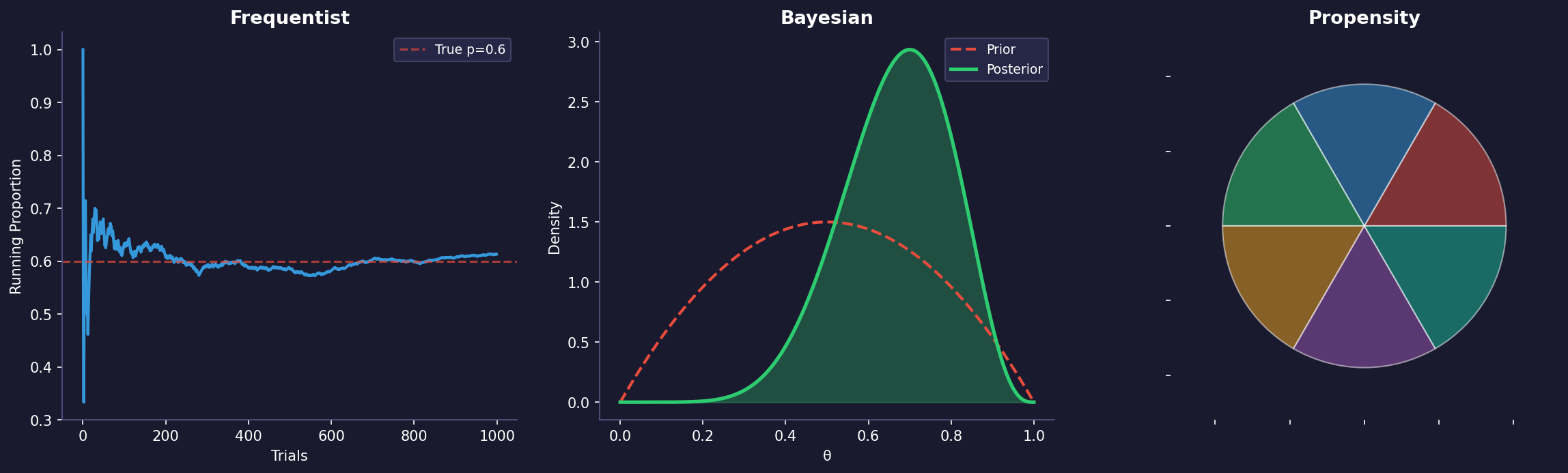
When we think about probability, there are three main philosophical approaches: frequentist, Bayesian, and propensity. Each offers a different lens for understanding uncertainty and probability.

The Scenario #

Imagine we’re dealing with a new diagnostic test for a rare genetic condition that affects 1 in 1000 people. The test has the following characteristics:

If someone has the condition, the test will be positive 99% of the time (sensitivity)
If someone doesn’t have the condition, the test will be negative 95% of the time (specificity)

Now, let’s say Sarah gets tested and receives a positive result. What’s the probability that she actually has the condition? Each probability paradigm approaches this question differently.

The Frequentist Approach #

The frequentist views probability as the long-run frequency of events in repeated trials. They might say:

“If we were to run this test on a very large number of people, and look only at the positive test results, what proportion of those people would actually have the condition?”

The frequentist would focus on the sampling distribution and confidence intervals. They might resist making a direct probability statement about Sarah’s individual case, arguing that she either has the condition or doesn’t – there’s no probability about it. Instead, they would frame their analysis in terms of error rates and long-term frequencies.

In this case, they would calculate the false positive and true positive rates across a hypothetical population:

In 1000 people, 1 person would have the condition
That 1 person would test positive 99% of the time = 0.99 true positives
The 999 people without the condition would test positive 5% of the time = 49.95 false positives
Total positive tests = 50.94
Proportion of positive tests that are true positives ≈ 1.94%

The Bayesian Approach #

The Bayesian sees probability as a degree of belief that gets updated with new evidence. They would start with a prior probability (the base rate of 1/1000) and update it with the new evidence (the positive test result) using Bayes’ Theorem.

The Bayesian would say: “Before the test, we believed Sarah had a 0.1% chance of having the condition. The positive test result gives us new information to update this belief.”

Using Bayes’ Theorem: P(Condition|Positive) = P(Positive|Condition) × P(Condition) / P(Positive) = 0.99 × 0.001 / (0.99 × 0.001 + 0.05 × 0.999) ≈ 0.0194 or about 1.94%

The Bayesian is comfortable making a direct probability statement about Sarah ‘s specific case, saying there’s a 1.94% chance she has the condition.

The Propensity Approach #

The propensity theorist views probability as an objective physical property – a tendency or disposition of a system to produce certain outcomes. They might say:

“The test result reflects the physical properties of Sarah’s genes and the testing mechanism. The probability emerges from the actual physical setup of the situation.”

They would focus on the causal mechanisms involved: the biological factors that cause the condition, the chemical reactions in the test, and how these physical properties interact to produce results. They might analyze the molecular basis of the test’s accuracy and how it interacts with the genetic markers it’s designed to detect.

These different approaches can lead to different practical recommendations:

A frequentist might emphasize the need for additional testing, pointing out that in a large population, most positive results are false positives.
A Bayesian might focus on gathering more prior information about Sarah (family history, symptoms, etc.) to refine the probability estimate.
A propensity theorist might advocate for understanding the biological mechanism better, perhaps recommending a different type of test that targets the condition’s physical manifestations more directly.

The formal backbone all three share #

What I find interesting is that the three camps disagree about what probability means, but they all use the same mathematics. Here is that common core, with Sarah’s numbers plugged in.

Kolmogorov’s axioms #

A probability space is a triple $(\Omega, \mathcal{F}, \mathbb{P})$. $\Omega$ is the set of outcomes, $\mathcal{F}$ is a $\sigma$-algebra of events (subsets of $\Omega$ closed under complement and countable union), and $\mathbb{P} : \mathcal{F} \to \mathbb{R}$ satisfies

Non-negativity: $\mathbb{P}(A) \ge 0$ for every $A \in \mathcal{F}$.
Normalisation: $\mathbb{P}(\Omega) = 1$.
Countable additivity: if $A_1, A_2, \dots$ are pairwise disjoint, then $\mathbb{P}\big(\bigcup_i A_i\big) = \sum_i \mathbb{P}(A_i)$.

The axioms say nothing about whether $\mathbb{P}$ is a frequency, a belief or a propensity. That neutrality is why they are shared, and why the debate above is about interpretation and not about mathematics.

Conditional probability and Bayes’ theorem #

For $\mathbb{P}(B) > 0$, the conditional probability is defined as $\mathbb{P}(A \mid B) = \mathbb{P}(A \cap B)/\mathbb{P}(B)$. If $A_1, \dots, A_k$ partition $\Omega$, the law of total probability is $\mathbb{P}(B) = \sum_j \mathbb{P}(B \mid A_j)\,\mathbb{P}(A_j)$. Writing $\mathbb{P}(A \cap B)$ in two ways gives Bayes’ theorem:

$$\mathbb{P}(A \mid B) = \frac{\mathbb{P}(B \mid A)\,\mathbb{P}(A)}{\mathbb{P}(B)} .$$

For Sarah, let $C$ be “has the condition” and $+$ be “tests positive”. Then $\mathbb{P}(C) = 0.001$, the sensitivity is $\mathbb{P}(+ \mid C) = 0.99$, and the false positive rate is $\mathbb{P}(+ \mid \bar{C}) = 1 - 0.95 = 0.05$:

$$\mathbb{P}(C \mid +) = \frac{0.99 \times 0.001}{0.99 \times 0.001 + 0.05 \times 0.999} = \frac{0.00099}{0.05094} \approx 0.0194 .$$

The odds form is the cleanest way I know to see what the test does:

$$\underbrace{\frac{\mathbb{P}(C \mid +)}{\mathbb{P}(\bar C \mid +)}}_{\text{posterior odds}} = \underbrace{\frac{\mathbb{P}(+ \mid C)}{\mathbb{P}(+ \mid \bar C)}}_{\text{likelihood ratio} \,=\, 19.8} \times \underbrace{\frac{\mathbb{P}(C)}{\mathbb{P}(\bar C)}}_{\text{prior odds} \,=\, 1/999} .$$

A positive result multiplies the odds by about 20. But the starting odds are 1 to 999, so the result is still only about 1 to 50. It also makes the frequentist’s “test again” advice concrete. If a second test is positive and, given the true status, independent of the first, the odds are multiplied by $19.8$ again: $19.8^2/999 \approx 0.39$, so $\mathbb{P}(C \mid +, +) \approx 0.28$.

Law of large numbers: where “long-run frequency” comes from #

The frequentist’s definition shows up inside the axioms as a theorem. Let $X_1, X_2, \dots$ be independent and identically distributed with $\mathbb{E}|X_1| < \infty$, and let $\bar X_n = \frac{1}{n}\sum_{i=1}^n X_i$. The strong law of large numbers says

$$\bar X_n \xrightarrow{\text{a.s.}} \mathbb{E}[X_1] \quad \text{as } n \to \infty .$$

Take $X_i = \mathbf{1}\{\text{person } i \text{ tests positive}\}$, an indicator with $\mathbb{E}[X_i] = p$. Then the observed fraction of positives converges to $p$ with probability one. The “1000 people” table above is this theorem used at a finite $n$.

Central limit theorem: how fast, and the confidence interval #

If in addition $\sigma^2 = \operatorname{Var}(X_1) < \infty$, the central limit theorem says

$$\sqrt{n}\,\big(\bar X_n - \mathbb{E}[X_1]\big) \xrightarrow{d} \mathcal{N}(0, \sigma^2) .$$

For the indicator, $\sigma^2 = p(1-p)$, and that is the frequentist’s error bar. Suppose the specificity was estimated by testing $n = 2000$ healthy people and $100$ came back positive. The estimated false positive rate is $\hat p = 0.05$, and the approximate 95% confidence interval is

$$\hat p \pm 1.96\sqrt{\frac{\hat p (1 - \hat p)}{n}} = 0.05 \pm 0.0096 .$$

The interval is a statement about the procedure: about 95% of intervals built this way contain the true $p$. It is not a statement about this particular $p$.

The Bayesian handles the same data with a prior. With a uniform $\mathrm{Beta}(1, 1)$ prior on $p$, observing $100$ positives in $2000$ gives the posterior $\mathrm{Beta}(101, 1901)$, with mean $101/2002 \approx 0.0504$. The Bernstein-von Mises theorem says that, under regularity conditions, such a posterior approaches $\mathcal{N}\big(\hat p, \hat p(1-\hat p)/n\big)$ as $n$ grows. So with lots of data the 95% credible interval and the 95% confidence interval nearly coincide. The two camps end up with the same numbers and keep arguing about what they mean.

The propensity view has no separate formalism. It is an account of what makes $\mathbb{P}(+ \mid C) = 0.99$ true. One known complication is Humphreys’ paradox: Bayes lets us invert $\mathbb{P}(+ \mid C)$ into $\mathbb{P}(C \mid +)$, but the test result does not cause the condition. So it is unclear what physical tendency the inverted probability would describe.

References #

1. 1. Kolmogorov (1933). Grundbegriffe der Wahrscheinlichkeitsrechnung. Springer. English translation: Foundations of the Theory of Probability (1950), Chelsea.
1. Durrett (2019). Probability: Theory and Examples, 5th ed. Cambridge University Press.
1. 1. Popper (1959). The Propensity Interpretation of Probability. The British Journal for the Philosophy of Science 10(37), 25–42.
1. Humphreys (1985). Why Propensities Cannot be Probabilities. The Philosophical Review 94(4), 557–570.
1. Hájek. Interpretations of Probability. The Stanford Encyclopedia of Philosophy.

Related posts

Comments