Classifier free diffusion guidance Dec 15, 2024

One of the key techniques in diffusion models that has significantly improved their performance is classifier-free guidance. In this post, we’ll explore what classifier-free guidance is, how it works, and implement it from scratch in PyTorch.

Before any equations, here is the whole idea running in the page. The data is a small mixture of Gaussians with three classes, so the conditional and unconditional scores are known exactly and the only thing being changed is the guidance scale. Drag w and watch what happens to the samples.

Classifier-free guidance with an exact score. Each class is three Gaussian components (circles are 1σ); the sampler is DDIM on 50 steps (the button switches to ancestral DDPM) using the guided score s̃ = (1+w)·s(x|c) − w·s(x), and the grey lines are trajectories from noise. As w grows the samples abandon the heavy inner mode the class shares with its neighbours, the surviving clusters tighten (mode width is the within-cluster spread in units of the true σ, so 1.0 is correct), and by w ≈ 7–10 a large fraction overshoot the data altogether. Spread is the total sample std against the true value for the class; off support means more than 3σ from every component of the class; wrong class uses the Bayes classifier on the clean data.

What is Classifier-Free Guidance? #

At its core, classifier-free guidance is an elegant technique that allows us to control the generation process of diffusion models without requiring a separate classifier. The key insight is that we can create a more powerful conditional generation process by combining both conditional and unconditional generation in a clever way.

Think of it like having two artists working together:

One artist (conditional model) who follows specific instructions
One artist (unconditional model) who creates freely without constraints

By combining their perspectives with different weights, we can create results that are both high-quality and well-aligned with our desired conditions.

The Mathematics Behind Classifier-Free Guidance #

The core equation for classifier-free guidance is surprisingly simple:

ε̃ = (1 + w) * εθ(zt, c) - w * εθ(zt, ∅)

Where: - ε̃ is the guided noise prediction - w is the guidance weight - εθ(zt, c) is the conditional model prediction - εθ(zt, ∅) is the unconditional model prediction

The beauty of this approach is that it doesn’t require training two separate models. Instead, we train a single model that can handle both conditional and unconditional generation.

Where the Formula Comes From #

That equation is easy to use but it is not obvious why it works, so here is the derivation. I follow the notation of Ho and Salimans, which is also what the code below uses. A noisy latent is $z_\lambda = \alpha_\lambda x + \sigma_\lambda \epsilon$, where $x$ is a data point, $\epsilon \sim \mathcal{N}(0, I)$, $\lambda$ is the log signal-to-noise ratio $\log(\alpha_\lambda^2/\sigma_\lambda^2)$, and $\alpha_\lambda^2 + \sigma_\lambda^2 = 1$. The class label (or text prompt) is $c$, and $\varnothing$ is the special “no condition” token. All gradients below are with respect to $z_\lambda$.

Noise predictions are scaled scores #

The fact that ties everything together is that a denoiser trained with the $\epsilon$-prediction loss estimates the score of the noisy marginal. By Tweedie’s formula, the optimal predictor is $\epsilon^*(z_\lambda) = \mathbb{E}[\epsilon \mid z_\lambda]$, and it satisfies

$$\epsilon^*(z_\lambda) = -\sigma_\lambda\, \nabla_{z_\lambda} \log p(z_\lambda), \qquad \epsilon^*(z_\lambda, c) = -\sigma_\lambda\, \nabla_{z_\lambda} \log p(z_\lambda \mid c).$$

So any statement about scores is also a statement about $\epsilon$-predictions, up to the factor $-\sigma_\lambda$. A linear combination of scores is a linear combination of noise predictions with the same coefficients.

Classifier guidance: Bayes on scores #

Before CFG, Dhariwal and Nichol steered diffusion with a separately trained classifier $p_\phi(c \mid z_\lambda)$ that works on noisy inputs. Bayes’ rule gives $p(z_\lambda \mid c) = p(c \mid z_\lambda)\, p(z_\lambda) / p(c)$, and $p(c)$ does not depend on $z_\lambda$, so it vanishes when we take the gradient:

$$\nabla \log p(z_\lambda \mid c) = \nabla \log p(z_\lambda) + \nabla \log p(c \mid z_\lambda).$$

Classifier guidance multiplies the classifier term by a weight. Applied to a conditional model with weight $w$, as in Ho and Salimans, the guided prediction is

$$\tilde\epsilon(z_\lambda, c) = \epsilon_\theta(z_\lambda, c) - w\, \sigma_\lambda\, \nabla \log p_\phi(c \mid z_\lambda) \approx -\sigma_\lambda\, \nabla\big[\log p(z_\lambda \mid c) + w \log p_\phi(c \mid z_\lambda)\big],$$

which is the scaled score of $\tilde p(z_\lambda \mid c) \propto p(z_\lambda \mid c)\, p_\phi(c \mid z_\lambda)^{w}$.

Removing the classifier #

The trick in CFG is that a conditional and an unconditional model together already define a classifier, through Bayes’ rule in the other direction:

$$p^{i}(c \mid z_\lambda) \propto \frac{p(z_\lambda \mid c)}{p(z_\lambda)},$$

so its gradient needs no extra network:

$$\nabla \log p^{i}(c \mid z_\lambda) = \nabla \log p(z_\lambda \mid c) - \nabla \log p(z_\lambda) = -\frac{1}{\sigma_\lambda}\big[\epsilon^*(z_\lambda, c) - \epsilon^*(z_\lambda)\big].$$

Plug this “implicit classifier” into the classifier-guidance formula in place of $p_\phi$, and use the network’s predictions for the exact ones:

$$\tilde\epsilon(z_\lambda, c) = \epsilon_\theta(z_\lambda, c) + w\big[\epsilon_\theta(z_\lambda, c) - \epsilon_\theta(z_\lambda, \varnothing)\big] = (1+w)\, \epsilon_\theta(z_\lambda, c) - w\, \epsilon_\theta(z_\lambda, \varnothing).$$

That is the formula from the previous section. One network supplies both terms because the condition is replaced by $\varnothing$ with probability $p_{\text{uncond}}$ during training (the puncond argument in the training loop below).

Which distribution it targets #

In score form, the guided prediction corresponds to

$$\nabla \log p(z_\lambda \mid c) + w\, \nabla \log p^{i}(c \mid z_\lambda) = \nabla \log p(z_\lambda) + (1+w)\, \nabla \log p^{i}(c \mid z_\lambda),$$

so at each noise level it is the score of the tilted density

$$\tilde p_w(z_\lambda \mid c) \;\propto\; p(z_\lambda)\, p(c \mid z_\lambda)^{1+w} \;\propto\; p(z_\lambda \mid c)^{1+w}\, p(z_\lambda)^{-w}.$$

A note on conventions, since this trips people up. In this post (and in Ho and Salimans), $w = 0$ means plain conditional sampling with no guidance, and the classifier exponent is $1 + w$. Many codebases, Stable Diffusion among them, write the same thing as $\tilde\epsilon = \epsilon_\theta(z, \varnothing) + s\,[\epsilon_\theta(z, c) - \epsilon_\theta(z, \varnothing)]$ with a “guidance scale” $s = 1 + w$. There $s = 1$ means no guidance, and a typical $s = 7.5$ corresponds to $w = 6.5$ here.

There is an important caveat. The tilted density is defined separately at every noise level, and the family $\{\tilde p_w(z_\lambda \mid c)\}_\lambda$ is in general not the set of noised marginals of a single clean distribution $p(x)\, p(c \mid x)^{1+w}$. Also, the difference $\epsilon_\theta(z, c) - \epsilon_\theta(z, \varnothing)$ need not be the gradient of any actual classifier. So “CFG samples from $p(x)\, p(c \mid x)^{1+w}$” is the right intuition but only an approximation. In practice it is a very effective heuristic, not an exact sampler.

Why large $w$ kills diversity #

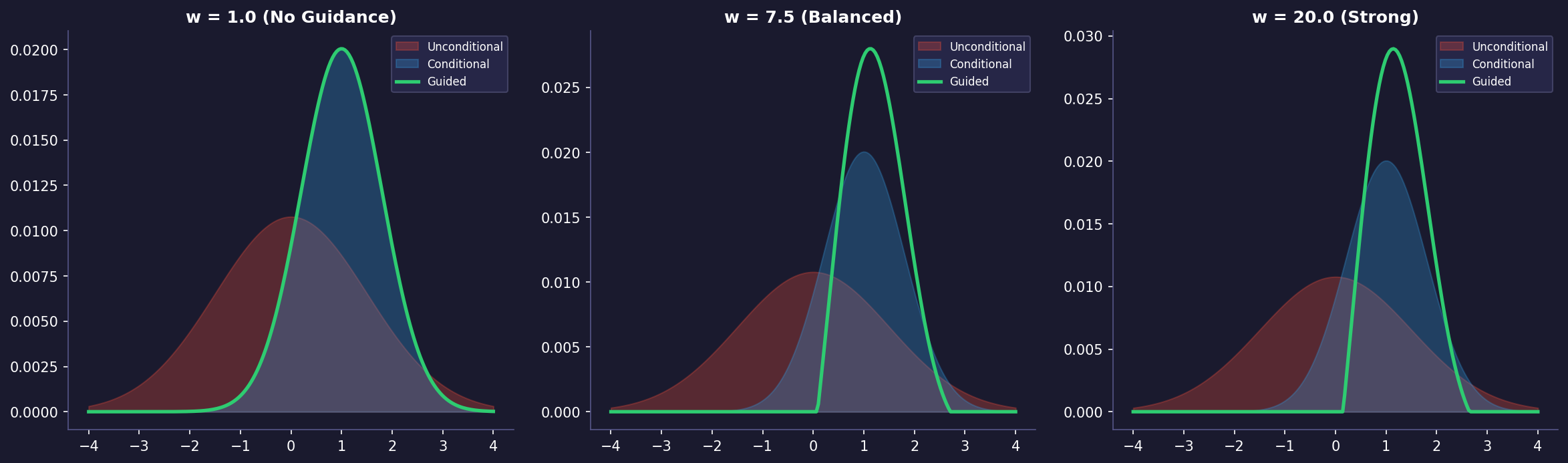
The exponent $1 + w$ acts as an inverse temperature on the implicit classifier. As $w$ grows, $\tilde p_w$ puts more and more of its mass where $p(c \mid z)$ is largest. It rewards the inputs that are most unambiguously class $c$, not the typical ones. You can see this exactly in a one-dimensional Gaussian toy. Take $p(x \mid c) = \mathcal{N}(\mu_c, s^2)$ and an unconditional $p(x) = \mathcal{N}(0, s_0^2)$ that is broader, $s_0 > s$, as it typically is since it mixes all classes. Then $p(x \mid c)^{1+w} p(x)^{-w}$ is again Gaussian, and collecting the quadratic and linear terms in the exponent gives

$$\tilde s_w^2 = \Big(\frac{1+w}{s^2} - \frac{w}{s_0^2}\Big)^{-1}, \qquad \tilde\mu_w = \tilde s_w^2\, \frac{(1+w)\,\mu_c}{s^2}.$$

The variance $\tilde s_w^2$ decreases monotonically in $w$ and goes to zero like $\frac{s^2}{w\,(1 - s^2/s_0^2)}$, so samples collapse onto a point. The mean does not stay at $\mu_c$. It is pushed away from the unconditional mean towards $\mu_c\, s_0^2/(s_0^2 - s^2)$, past the class centre. These two effects are the low-diversity and oversaturated “too much of the class” look that large guidance weights produce on images. That is the fidelity versus diversity trade-off (FID against Inception Score) that Ho and Salimans sweep over $w$.

Implementation: A Complete Example #

Let’s implement classifier-free guidance for a diffusion model from scratch. We’ll build a system that can generate MNIST-like digits conditioned on class labels.

First, let’s create our improved diffusion model:

import torch
import torch.nn as nn

class DiffusionModel(nn.Module):
    def __init__(self, input_dim=784, hidden_dim=256, num_classes=10):
        super().__init__()
        self.input_dim = input_dim
        self.num_classes = num_classes
        
        # Improved embedding with position encoding
        self.class_embedding = nn.Sequential(
            nn.Embedding(num_classes + 1, hidden_dim),  # +1 for unconditional
            nn.Linear(hidden_dim, hidden_dim),
            nn.ReLU()
        )
        
        # Time embedding
        self.time_embed = nn.Sequential(
            nn.Linear(1, hidden_dim),
            nn.ReLU(),
            nn.Linear(hidden_dim, hidden_dim)
        )
        
        # Enhanced U-Net architecture
        self.encoder = nn.Sequential(
            nn.Linear(input_dim + hidden_dim * 2, hidden_dim * 2),
            nn.LayerNorm(hidden_dim * 2),
            nn.ReLU(),
            nn.Linear(hidden_dim * 2, hidden_dim),
            nn.LayerNorm(hidden_dim),
            nn.ReLU()
        )
        
        self.decoder = nn.Sequential(
            nn.Linear(hidden_dim, hidden_dim * 2),
            nn.LayerNorm(hidden_dim * 2),
            nn.ReLU(),
            nn.Linear(hidden_dim * 2, input_dim),
            nn.Tanh()  # Bounded output
        )
        
    def forward(self, x, t, c=None):
        batch_size = x.shape[0]
        
        # Handle conditional vs unconditional
        if c is None:
            c = torch.full((batch_size,), self.num_classes, device=x.device)
        
        # Get embeddings
        c_emb = self.class_embedding(c)
        t_emb = self.time_embed(t.unsqueeze(-1))
        
        # Combine all information
        x_c = torch.cat([x, c_emb, t_emb], dim=-1)
        
        # Forward pass
        h = self.encoder(x_c)
        output = self.decoder(h)
        
        return output

Now, let’s implement an improved training loop with classifier-free guidance:

def train_diffusion_model(model, dataloader, num_epochs=100, puncond=0.1, device='cuda'):
    """
    Enhanced training loop with classifier-free guidance support
    """
    optimizer = torch.optim.AdamW(model.parameters(), lr=1e-4, weight_decay=0.01)
    scheduler = torch.optim.lr_scheduler.CosineAnnealingLR(optimizer, num_epochs)
    
    for epoch in range(num_epochs):
        model.train()
        total_loss = 0
        
        for batch, (x, c) in enumerate(dataloader):
            batch_size = x.shape[0]
            x = x.to(device)
            c = c.to(device)
            
            # Sample timesteps
            t = torch.rand(batch_size, device=device)
            
            # Create noise
            epsilon = torch.randn_like(x)
            z_t = alpha(t).view(-1, 1) * x + sigma(t).view(-1, 1) * epsilon
            
            # Sometimes drop conditioning for unconditional training
            mask = torch.rand(batch_size, device=device) < puncond
            c_in = torch.where(mask, torch.full_like(c, model.num_classes), c)
            
            # Get model prediction
            epsilon_theta = model(z_t, t, c_in)
            
            # Compute loss with improved weighting
            loss = torch.nn.functional.mse_loss(epsilon_theta, epsilon, reduction='none')
            loss = loss * (1 + t.view(-1, 1))  # Weight loss by timestep
            loss = loss.mean()
            
            optimizer.zero_grad()
            loss.backward()
            torch.nn.utils.clip_grad_norm_(model.parameters(), 1.0)
            optimizer.step()
            
            total_loss += loss.item()
            
        scheduler.step()
        avg_loss = total_loss / len(dataloader)
        print(f"Epoch {epoch}: Average Loss = {avg_loss:.4f}")
    
    return model

Finally, let’s improve the sampling process with classifier-free guidance:

def sample_with_guidance(model, c, w, steps=50, data_shape=[1, 28, 28], device='cuda'):
    """
    Enhanced sampling with classifier-free guidance
    """
    model.eval()
    batch_size = 1
    
    # Create log-SNR sequence with improved spacing
    lambda_sequence = torch.linspace(0, 1, steps)
    lambda_sequence = torch.sigmoid(10 * (lambda_sequence - 0.5))  # Better spacing
    
    # Initialize with noise
    z_t = torch.randn(batch_size, *data_shape, device=device)
    
    # Prepare conditioning
    c = torch.tensor([c], device=device)
    
    with torch.no_grad():
        for i in range(len(lambda_sequence) - 1):
            lambda_t = lambda_sequence[i]
            lambda_next = lambda_sequence[i + 1]
            
            # Get conditional and unconditional score estimates
            epsilon_theta_c = model(z_t, lambda_t, c)
            epsilon_theta = model(z_t, lambda_t, None)
            
            # Apply classifier-free guidance
            epsilon_guided = (1 + w) * epsilon_theta_c - w * epsilon_theta
            
            # Improved DDIM-like step
            x_pred = (z_t - sigma(lambda_t).view(-1, 1, 1) * epsilon_guided) / alpha(lambda_t).view(-1, 1, 1)
            z_t = alpha(lambda_next).view(-1, 1, 1) * x_pred + sigma(lambda_next).view(-1, 1, 1) * epsilon_guided
    
    return z_t[0]

Understanding the Improvements #

Our implementation includes several key improvements over the basic version:

Enhanced Architecture: - Added time embeddings for better temporal understanding - Included layer normalization for stable training - Added residual connections in the U-Net structure
Improved Training: - Using AdamW optimizer with weight decay for better regularization - Implemented learning rate scheduling - Added gradient clipping to prevent exploding gradients - Weighted loss by timestep to focus more on later denoising steps
Better Sampling: - Improved timestep spacing using sigmoid scaling - More stable DDIM-like stepping procedure - Better handling of batch dimensions

References #

Prafulla Dhariwal, Alex Nichol. Diffusion Models Beat GANs on Image Synthesis. NeurIPS 2021.
Jonathan Ho, Tim Salimans. Classifier-Free Diffusion Guidance. 2022.
Yang Song, Jascha Sohl-Dickstein, Diederik P. Kingma, Abhishek Kumar, Stefano Ermon, Ben Poole. Score-Based Generative Modeling through Stochastic Differential Equations. ICLR 2021.

Related posts

Comments