Diffusion models for time series
On this post I will explore the main findings from the paper “UTSD: Unified Time Series Diffusion Model” and an explanation of the content. For more details here is the link to the paper Link to paper
Summary of Findings from UTSD Paper #
The authors of the paper propose a novel architecture, UTSD, for time series analysis. The researchers note the prevalence of time series data in a variety of real world applications. They also point out that data across different domains often have different statistical properties. They posit that this creates a challenge to the generalizability and robustness of time series analysis. In order to address this, the authors propose a unified time series diffusion model. The paper explains that the UTSD model uses a diffusion denoising process, in contrast to autoregressive models, to model the mixture distribution of cross-domain data and generate a prediction sequence for the target domain. The model learns from time series data across a range of domains with the goal of having strong generalization capabilities and robustness to achieve zero-shot inference on unseen domains. UTSD consists of three key designs:
- Condition-denoising architecture
- Reverse noise reduction process in the actual sequence space
- Conditional generation strategy based on improved classifier-free guidance
The paper reports that UTSD outperforms existing foundation models on all data domains. It achieves an average MSE reduction of 14.2%, 20.1%, and 27.6% compared to the existing Moirai, UniTime, and GPT4TS, respectively. The paper also reports that UTSD, when trained from scratch, achieves comparable performance to domain-specific models. In the paper, the authors contend that UTSD shows stable and reliable time series generation which indicates the model’s potential as a foundational model for time series analysis.
Explanation of the Paper #
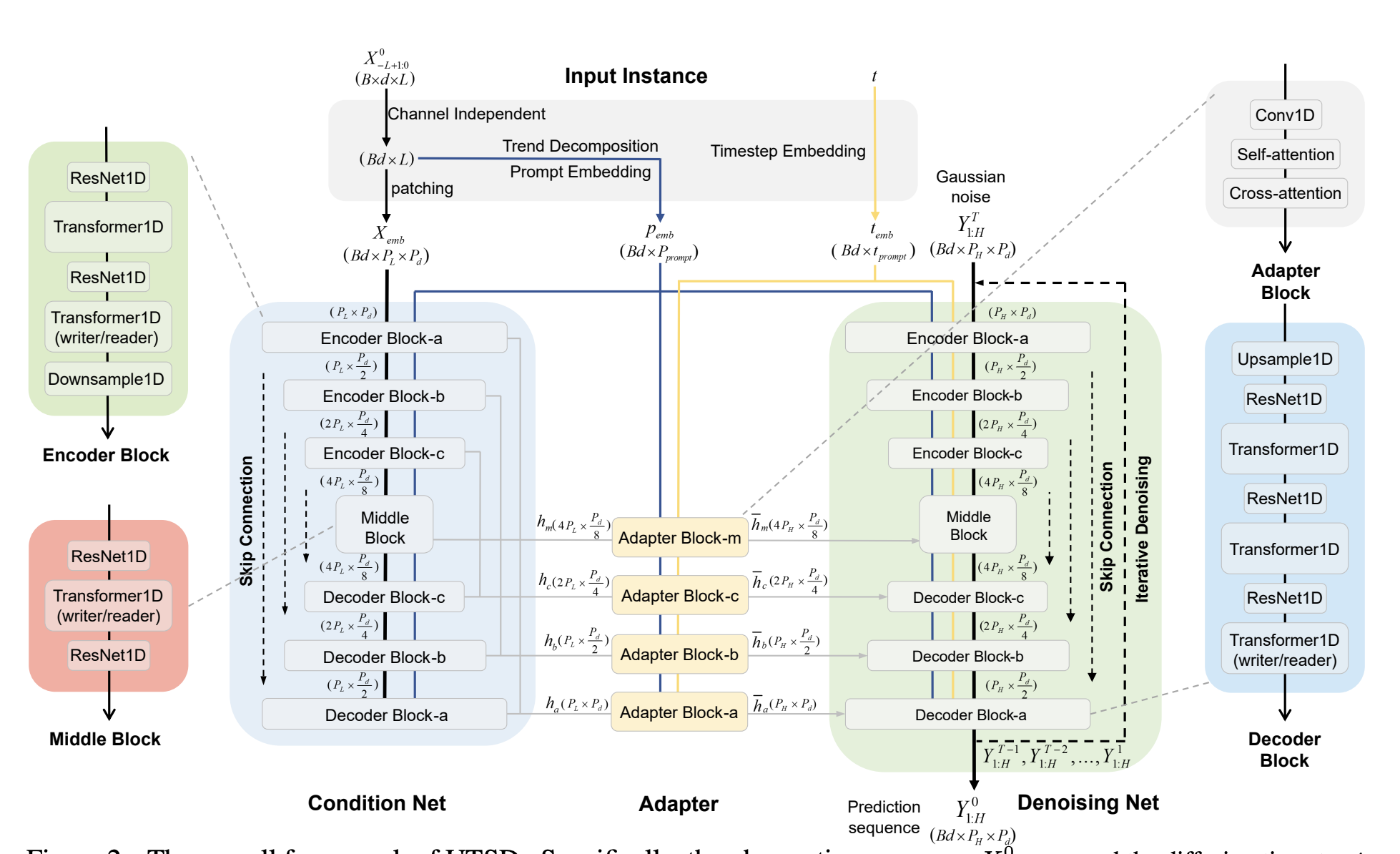
The paper presents a detailed explanation of the UTSD model architecture and its three key design elements. These designs aim to address the challenges of modeling probability distributions across multiple time series domains and generating accurate long-term forecasts.
1. Condition-Denoising Architecture #
This architecture includes a Condition Net and a Denoising Net. The Condition Net learns multi-scale representations of temporal fluctuation patterns from different time series domains. These representations are then used as conditional variables to guide the Denoising Net in generating the prediction sequence. The paper argues that capturing multi-scale representations is crucial because time series from various domains often exhibit different latent patterns.
2. Reverse Noise Reduction in Actual Sequence Space #
UTSD performs the reverse noise reduction process directly in the actual sequence space, unlike traditional diffusion models that operate in a latent space. This design choice is justified by the fact that iterative denoising in the latent space can lead to error accumulation, which is amplified when aligning the latent space back to the actual sequence space.
3. Improved Classifier-Free Guidance #
The UTSD model uses an improved classifier-free guidance strategy to ensure strong generalization ability. This strategy leverages the multi-scale representation captured by the Condition Net as a conditional variable to guide the reconstruction of the forecast from Gaussian noise.
Additional Architectural Components #
- Transfer-Adapter Module: This module allows for efficient fine-tuning of the pre-trained UTSD model on specific downstream tasks. It transforms the fluctuation patterns learned during pre-training into the latent space of the target domain, enabling the generation of domain-specific time series samples.
- Blocks Implementation: The Condition Net and Denoising Net are built using ResNet1D and Transformer1D modules. The ResNet1D modules handle the embedding of diffusion timesteps and latent representations, while the Transformer1D modules capture dependencies within the observation sequence and leverage historical fluctuation patterns as context for denoising.
How Conditioning Enters the Reverse Process #
The three designs above all answer one question: how does the observed part of a series steer the denoiser? UTSD is one answer. Here I want to write the general machinery as equations, following CSDI (Tashiro et al.), which states it most cleanly. I use DDPM notation for the noise schedule: $\beta_t$, $\alpha_t = 1 - \beta_t$, $\bar\alpha_t = \prod_{s \le t}\alpha_s$. Note that CSDI itself writes $\alpha_t$ for the cumulative product.
Targets and conditional observations #
Take a multivariate series $x_0 \in \mathbb{R}^{K \times L}$ ($K$ channels, $L$ time steps), and split its entries into two disjoint sets.
- Conditional observations $x_0^{co}$ are the values we know.
- Targets $x_0^{ta}$ are the values we want a distribution over.
Imputation and forecasting are the same problem with different masks. For imputation, the targets are the missing entries scattered through the window. For forecasting, they are every entry after the last observed time step, with the history as $x_0^{co}$.
The conditional reverse process #
Only the targets are diffused. The forward process is the usual one applied to $x_0^{ta}$, so $x_t^{ta} = \sqrt{\bar\alpha_t}\, x_0^{ta} + \sqrt{1-\bar\alpha_t}\,\epsilon$. The reverse process is conditioned on the clean observations at every step:
$$p_\theta\big(x_{0:T}^{ta} \mid x_0^{co}\big) = p\big(x_T^{ta}\big) \prod_{t=1}^{T} p_\theta\big(x_{t-1}^{ta} \mid x_t^{ta}, x_0^{co}\big), \qquad x_T^{ta} \sim \mathcal{N}(0, I),$$
$$p_\theta\big(x_{t-1}^{ta} \mid x_t^{ta}, x_0^{co}\big) = \mathcal{N}\Big(x_{t-1}^{ta};\ \mu_\theta\big(x_t^{ta}, t \mid x_0^{co}\big),\ \sigma_t^2 I\Big).$$
The mean keeps exactly the DDPM form. Only the noise predictor gains an extra input:
$$\mu_\theta\big(x_t^{ta}, t \mid x_0^{co}\big) = \frac{1}{\sqrt{\alpha_t}}\Big(x_t^{ta} - \frac{\beta_t}{\sqrt{1-\bar\alpha_t}}\, \epsilon_\theta\big(x_t^{ta}, t \mid x_0^{co}\big)\Big).$$
Training is the simple $\epsilon$-loss, conditioned:
$$\mathcal{L}(\theta) = \mathbb{E}_{x_0,\ \epsilon \sim \mathcal{N}(0, I),\ t}\Big[\big\|\epsilon - \epsilon_\theta\big(\sqrt{\bar\alpha_t}\, x_0^{ta} + \sqrt{1-\bar\alpha_t}\,\epsilon,\ t \mid x_0^{co}\big)\big\|^2\Big],$$
where $\epsilon$ has the shape of $x_0^{ta}$. By the same Tweedie argument as in the unconditional case, the optimal predictor is a scaled conditional score:
$$\epsilon^*\big(x_t^{ta}, t \mid x_0^{co}\big) = -\sqrt{1-\bar\alpha_t}\ \nabla_{x_t^{ta}} \log q\big(x_t^{ta} \mid x_0^{co}\big).$$
Here is a practical question: where do training targets come from when the true missing values are unknown? CSDI uses self-supervision, much like masked language modelling. Some observed entries are hidden and become $x_0^{ta}$, and the rest serve as $x_0^{co}$. The masks are chosen at random, copied from missingness patterns found elsewhere in the data, or set to “the future” for forecasting.
Why condition on clean observations #
The alternative is to train an unconditional model of the full $x_0$ and impute by replacement. At each reverse step you would overwrite the known coordinates with a forward-noised copy $x_t^{co} = \sqrt{\bar\alpha_t}\, x_0^{co} + \sqrt{1-\bar\alpha_t}\,\epsilon'$. That approximates the conditional score with $\nabla_{x_t^{ta}} \log p(x_t^{ta}, x_t^{co})$, i.e. a score conditioned on noisy observations. Since $x_t^{co}$ is a corrupted version of $x_0^{co}$, it carries less information about the targets. CSDI argues that this noise can destroy useful information in the observations, and models $p(x_{t-1}^{ta} \mid x_t^{ta}, x_0^{co})$ directly. As I read it, UTSD’s Condition Net follows the same pattern: the history enters the denoiser as a representation $c = f_\psi(x_0^{co})$ of the clean observations, where $f_\psi$ is the Condition Net with parameters $\psi$, and not as a noised input.
Autoregressive forecasting #
TimeGrad (Rasul et al.) conditions differently. Time-series steps are generated one at a time, and the history is summarized by a recurrent state. To avoid a clash of indices, write $\tau$ for the time-series index and $n$ for the diffusion step. An RNN produces $h_{\tau-1}$ from the observations up to $\tau - 1$, and the loss at step $\tau$ is
$$\mathbb{E}_{x_\tau^0,\ \epsilon,\ n}\Big[\big\|\epsilon - \epsilon_\theta\big(\sqrt{\bar\alpha_n}\, x_\tau^0 + \sqrt{1-\bar\alpha_n}\,\epsilon,\ h_{\tau-1},\ n\big)\big\|^2\Big],$$
where $x_\tau^0$ is the clean value of the series at time $\tau$. Forecasting runs the reverse chain for $x_\tau$, feeds the sample back into the RNN, and repeats. That gives a joint distribution over the horizon through the chain rule. CSDI and UTSD instead denoise the whole target window at once.
Guidance on top of the condition #
Finally, the classifier-free guidance used by UTSD sits on top of this machinery. Bayes’ rule on scores gives
$$\nabla_{x_t^{ta}} \log p\big(x_t^{ta} \mid c\big) = \nabla_{x_t^{ta}} \log p\big(x_t^{ta}\big) + \nabla_{x_t^{ta}} \log p\big(c \mid x_t^{ta}\big).$$
Train one network with the condition randomly dropped to a null token $\varnothing$, and amplify the second term with a weight $w$:
$$\tilde\epsilon\big(x_t^{ta}, t, c\big) = (1+w)\,\epsilon_\theta\big(x_t^{ta}, t \mid c\big) - w\,\epsilon_\theta\big(x_t^{ta}, t \mid \varnothing\big).$$
Here $c$ is the multi-scale history representation from the Condition Net. UTSD’s “improved” variant modifies this basic recipe, and I refer to the paper for its exact form. The derivation of the basic formula, and of why large $w$ trades diversity for fidelity, is in my post on classifier-free guidance. For forecasting this matters directly: the spread of the sampled trajectories is the predictive uncertainty, so too much guidance gives overconfident prediction intervals.
References #
- Xiangkai Ma, Xiaobin Hong, Wenzhong Li, Sanglu Lu. UTSD: Unified Time Series Diffusion Model. 2024. (Later versions of the arXiv entry carry a different title.)
- Yusuke Tashiro, Jiaming Song, Yang Song, Stefano Ermon. CSDI: Conditional Score-based Diffusion Models for Probabilistic Time Series Imputation. NeurIPS 2021.
- Kashif Rasul, Calvin Seward, Ingmar Schuster, Roland Vollgraf. Autoregressive Denoising Diffusion Models for Multivariate Probabilistic Time Series Forecasting. ICML 2021.
- Jonathan Ho, Ajay Jain, Pieter Abbeel. Denoising Diffusion Probabilistic Models. NeurIPS 2020.
Comments