Flow Matching, a short overview
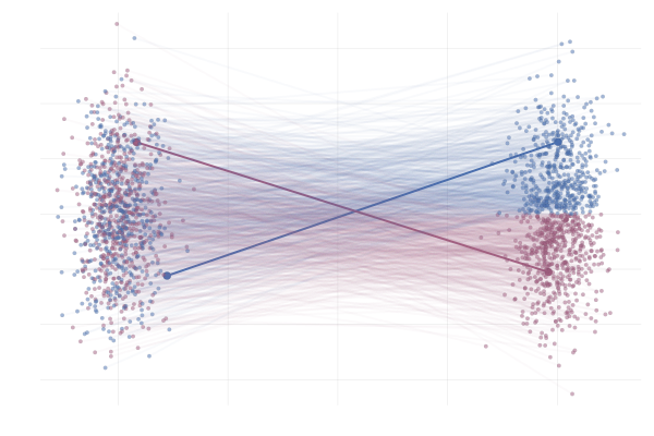
In summary, flow matching is a generative modeling technique that provides an elegant way to transform data distributions.
To make that concrete before the code, here is a flow running in the page: a Gaussian carried onto two moons. Nothing is trained; for a finite set of pairs the marginal velocity field has a closed form, so what you see is the exact flow, and the only thing that changes between the three options is how the noise and data points are paired and which path connects them.
import numpy as np
import torch
import torch.nn as nn
import torch.optim as optim

class FlowMatchingModel:
    def __init__(self, input_dim, hidden_dim):
        """
        Initialize Flow Matching Model

        Args:
            input_dim (int): Dimension of input data
            hidden_dim (int): Dimension of hidden layers
        """
        self.base_distribution = None  # Initial data distribution
        self.target_distribution = None  # Target data distribution

        # Neural network to learn the flow
        self.flow_network = nn.Sequential(
            nn.Linear(input_dim + 1, hidden_dim),  # +1 for time conditioning
            nn.ReLU(),
            nn.Linear(hidden_dim, hidden_dim),
            nn.ReLU(),
            nn.Linear(hidden_dim, input_dim)
        )

        self.optimizer = optim.Adam(self.flow_network.parameters())

    def sample_base_distribution(self, num_samples):
        """
        Sample from the base (initial) distribution

        Args:
            num_samples (int): Number of samples to generate

        Returns:
            torch.Tensor: Samples from base distribution
        """
        # Example: Gaussian distribution
        return torch.randn(num_samples, self.input_dim)

    def probability_flow_ode(self, x, t):
        """
        Compute the probability flow ODE

        Args:
            x (torch.Tensor): Current data point
            t (torch.Tensor): Time variable

        Returns:
            torch.Tensor: Flow direction
        """
        # Combine input and time as network input
        network_input = torch.cat([x, t], dim=1)
        return self.flow_network(network_input)

    def conditional_vector_field(self, x0, x1, t):
        """
        Compute the conditional vector field

        Args:
            x0 (torch.Tensor): Initial data point
            x1 (torch.Tensor): Target data point
            t (torch.Tensor): Time variable

        Returns:
            torch.Tensor: Conditional vector field
        """
        # Interpolate between source and target
        x_t = x0 * (1 - t) + x1 * t
        vector_field = x1 - x0
        return vector_field

    def loss_function(self, x0, x1):
        """
        Compute the flow matching loss

        Args:
            x0 (torch.Tensor): Initial data points
            x1 (torch.Tensor): Target data points

        Returns:
            torch.Tensor: Training loss
        """
        batch_size = x0.shape[0]
        t = torch.rand(batch_size, 1)  # Random time sampling

        # Compute vector field
        true_vector_field = self.conditional_vector_field(x0, x1, t)
        predicted_vector_field = self.probability_flow_ode(x0, t)

        # Compute MSE loss between true and predicted vector fields
        loss = torch.mean((predicted_vector_field - true_vector_field) ** 2)
        return loss

    def train(self, dataloader, epochs):
        """
        Train the Flow Matching Model

        Args:
            dataloader (torch.utils.data.DataLoader): Training data
            epochs (int): Number of training epochs
        """
        for epoch in range(epochs):
            for batch_x0, batch_x1 in dataloader:
                self.optimizer.zero_grad()
                loss = self.loss_function(batch_x0, batch_x1)
                loss.backward()
                self.optimizer.step()

            print(f"Epoch {epoch+1}/{epochs}, Loss: {loss.item()}")

    def generate_samples(self, num_samples):
        """
        Generate new samples using the learned flow

        Args:
            num_samples (int): Number of samples to generate

        Returns:
            torch.Tensor: Generated samples
        """
        # Start from base distribution and follow the learned flow
        x0 = self.sample_base_distribution(num_samples)

        # Perform sampling through ODE solving
        x_generated = x0  # Starting point
        time_steps = torch.linspace(0, 1, 100)

        for t in time_steps[1:]:
            vector_field = self.probability_flow_ode(x_generated, t)
            x_generated += vector_field * (time_steps[1] - time_steps[0])

        return x_generated

def main():
    # Hyperparameters
    input_dim = 10
    hidden_dim = 64
    num_epochs = 100

    flow_matching = FlowMatchingModel(input_dim, hidden_dim)
    flow_matching.train(dataloader, num_epochs)
    generated_samples = flow_matching.generate_samples(1000)
The math behind the code #
The code above is short, but each line rests on a derivation. In this section I want to go through them in order. I follow the convention of Lipman et al. and of the code: time runs from $t = 0$ to $t = 1$, $x_0 \sim p_0$ is a sample from a simple source (a standard Gaussian), and $x_1 \sim q$ is a data sample. All vectors live in $\mathbb{R}^d$.
Continuous normalizing flows #
A time-dependent vector field $v_t : \mathbb{R}^d \to \mathbb{R}^d$ defines a flow $\phi_t$ through the ODE
$$\frac{d}{dt}\phi_t(x) = v_t\big(\phi_t(x)\big), \qquad \phi_0(x) = x.$$
Pushing the source through the flow gives a path of densities
$p_t = [\phi_t]_{\#}\, p_0$, and we want $p_1 \approx q$. If $v_t$ is a neural
network $v_\theta(x, t)$, this is a continuous normalizing flow (CNF), which is
what probability_flow_ode and generate_samples implement. The second one is
an Euler solver.
The density along the path obeys the continuity equation, which says that probability mass is conserved as it is transported by $v_t$:
$$\partial_t p_t(x) + \nabla \cdot \big(p_t(x)\, v_t(x)\big) = 0.$$
From it we get the instantaneous change of variables of Chen et al. Follow a single trajectory $x(t) = \phi_t(x_0)$ and differentiate $\log p_t$ along it with the chain rule:
$$\frac{d}{dt}\log p_t\big(x(t)\big) = \frac{\partial_t p_t + \nabla p_t \cdot v_t}{p_t} = \frac{-\nabla\cdot(p_t v_t) + \nabla p_t \cdot v_t}{p_t} = -\nabla \cdot v_t\big(x(t)\big),$$
because $\nabla\cdot(p_t v_t) = \nabla p_t \cdot v_t + p_t\, \nabla\cdot v_t$. Integrating from $0$ to $1$:
$$\log p_1\big(x(1)\big) = \log p_0\big(x(0)\big) - \int_0^1 \operatorname{tr}\Big(\frac{\partial v_t}{\partial x}\big(x(t)\big)\Big)\, dt.$$
That is the CNF analogue of the $\log|\det J|$ term in a discrete normalizing flow. A determinant becomes a trace. In principle you can train a CNF by maximum likelihood with this formula, but every gradient step needs an ODE solve, plus a trace estimate (Hutchinson’s estimator, in FFJORD). That is slow, and it is the motivation for flow matching, which never simulates the ODE during training.
The flow-matching objective #
Suppose we had a target probability path $p_t$ with $p_0$ the source and $p_1 \approx q$, and a vector field $u_t$ that generates it (meaning the pair satisfies the continuity equation). Then we could simply regress:
$$\mathcal{L}_{\text{FM}}(\theta) = \mathbb{E}_{t \sim \mathcal{U}[0,1],\ x \sim p_t}\,\big\|v_\theta(x, t) - u_t(x)\big\|^2.$$
The problem is that we know neither $p_t$ nor $u_t$ in closed form. Lipman et al. solve it by building the path out of simple per-sample pieces. Let $z$ be some conditioning variable with distribution $q(z)$, and for each $z$ pick a conditional path $p_t(x \mid z)$ generated by a conditional field $u_t(x \mid z)$. Define the marginals
$$\begin{aligned} p_t(x) &= \int p_t(x \mid z)\, q(z)\, dz, \\ u_t(x) &= \int u_t(x \mid z)\, \frac{p_t(x \mid z)\, q(z)}{p_t(x)}\, dz = \mathbb{E}\big[u_t(x \mid z) \mid x_t = x\big]. \end{aligned}$$
The marginal field is the posterior average of the conditional fields. It really does generate the marginal path, because the continuity equation is linear:
$$\begin{aligned} \partial_t p_t(x) &= \int \partial_t p_t(x \mid z)\, q(z)\, dz = -\int \nabla\cdot\big(u_t(x \mid z)\, p_t(x \mid z)\big)\, q(z)\, dz \\ &= -\nabla\cdot\big(u_t(x)\, p_t(x)\big). \end{aligned}$$
Conditional flow matching with the linear path #
In the code, the conditioning variable is the pair $z = (x_0, x_1)$ with $x_0 \sim p_0$ and $x_1 \sim q$ drawn independently. The conditional path is the straight line between them, and its velocity is constant:
$$x_t = (1-t)\, x_0 + t\, x_1, \qquad u_t(x_t \mid x_0, x_1) = \frac{d x_t}{dt} = x_1 - x_0.$$
This is exactly conditional_vector_field. It is the $\sigma_{\min} \to 0$
limit of the “optimal transport” path of Lipman et al., who condition on $x_1$
alone and use $x_t = (1 - (1-\sigma_{\min})t)\, x_0 + t\, x_1$, with target
$x_1 - (1-\sigma_{\min})\, x_0$. It is also the interpolation used by rectified
flow. The conditional flow matching loss regresses on these per-pair targets:
$$\mathcal{L}_{\text{CFM}}(\theta) = \mathbb{E}_{t \sim \mathcal{U}[0,1],\ x_0 \sim p_0,\ x_1 \sim q}\, \big\|v_\theta\big((1-t)\,x_0 + t\,x_1,\ t\big) - (x_1 - x_0)\big\|^2.$$
One detail that matters when you implement it: the network must be evaluated at the interpolated point $x_t$, not at the endpoint $x_0$.
Why the CFM gradient equals the FM gradient #
At first sight the CFM loss is the wrong objective. A given point $x_t$ lies on many lines with different directions $x_1 - x_0$, so the regression target is noisy. The surprise is that it does not matter. Expand both squares (at a fixed $t$, then average over $t$):
$$\|v_\theta - u\|^2 = \|v_\theta\|^2 - 2\langle v_\theta, u\rangle + \|u\|^2.$$
- The $\|v_\theta\|^2$ term. In both losses $x$ is distributed as the marginal $p_t$, so $\mathbb{E}_{p_t(x)}\|v_\theta(x,t)\|^2 = \mathbb{E}_{q(z),\, p_t(x \mid z)}\|v_\theta(x,t)\|^2$.
- The cross term. Substitute the definition of $u_t$, which cancels the $p_t(x)$ in its denominator: $\mathbb{E}_{p_t(x)}\langle v_\theta(x,t), u_t(x)\rangle = \int \big\langle v_\theta(x,t), \int u_t(x \mid z)\, p_t(x \mid z)\, q(z)\, dz \big\rangle\, dx = \mathbb{E}_{q(z),\, p_t(x \mid z)}\langle v_\theta(x,t), u_t(x \mid z)\rangle.$
- The $\|u\|^2$ terms differ between the two losses, but neither depends on $\theta$.
Therefore $\mathcal{L}_{\text{FM}}(\theta) = \mathcal{L}_{\text{CFM}}(\theta) + C$ for a constant $C$, so $\nabla_\theta \mathcal{L}_{\text{FM}} = \nabla_\theta \mathcal{L}_{\text{CFM}}$. Equivalently, the minimizer of a squared loss is a conditional expectation, and here $\arg\min \mathcal{L}_{\text{CFM}}$ is $v^*(x, t) = \mathbb{E}[x_1 - x_0 \mid x_t = x] = u_t(x)$. The noise in the targets only adds variance to the stochastic gradient, not bias. Training is fully simulation-free: sample $t$, $x_0$, $x_1$, interpolate, regress.
Rectified flow and straightness #
The learned field is an average of straight-line velocities, so the ODE it defines is generally not straight. Where lines from different pairs cross, the average turns, and ODE trajectories cannot cross at all (solutions are unique). They bend and “rewire” which noise sample ends up at which data point. Curved trajectories are exactly what makes few-step Euler integration inaccurate.
Liu et al. measure this with the straightness of a flow $Z = \{Z_t\}$:
$$S(Z) = \int_0^1 \mathbb{E}\Big[\big\|(Z_1 - Z_0) - \dot Z_t\big\|^2\Big]\, dt.$$
$S(Z) = 0$ means every trajectory moves at constant velocity along a straight line. Then a single Euler step $Z_1 = Z_0 + v(Z_0, 0)$ is exact. Rectified flow improves straightness with reflow:
- Train $v^{(1)}$ with the CFM loss on independent pairs $(x_0, x_1)$.
- Draw $Z_0 \sim p_0$ and solve the learned ODE to get $Z_1$. The pair $(Z_0, Z_1)$ is a new coupling of $p_0$ and $p_1$ that is deterministic.
- Train $v^{(2)}$ with the same loss, but on the pairs $(Z_0, Z_1)$ instead of independent ones. Repeat if desired.
Each rectification preserves the marginals. Liu et al. also show that it never increases the transport cost $\mathbb{E}[c(Z_1 - Z_0)]$ for any convex $c$, and that iterating it drives the straightness towards zero. Since the new pairs are already matched by a flow with non-crossing paths, their connecting lines cross far less, the averaged field is closer to the per-pair one, and the ODE can be solved in one or a few steps. That is the basis of one-step rectified-flow samplers.
References #
- Ricky T. Q. Chen, Yulia Rubanova, Jesse Bettencourt, David Duvenaud. Neural Ordinary Differential Equations. NeurIPS 2018.
- Will Grathwohl, Ricky T. Q. Chen, Jesse Bettencourt, Ilya Sutskever, David Duvenaud. FFJORD: Free-form Continuous Dynamics for Scalable Reversible Generative Models. ICLR 2019.
- Yaron Lipman, Ricky T. Q. Chen, Heli Ben-Hamu, Maximilian Nickel, Matt Le. Flow Matching for Generative Modeling. ICLR 2023.
- Xingchao Liu, Chengyue Gong, Qiang Liu. Flow Straight and Fast: Learning to Generate and Transfer Data with Rectified Flow. ICLR 2023.
Comments