Scarf: Self Supervised Learning for Tabular Data
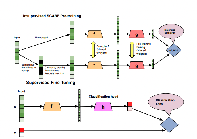
Machine learning often struggles with the scarcity of labeled data. While unlabeled datasets are abundant, obtaining high-quality labeled data remains expensive and time-consuming. SCARF emerges as a breakthrough methodology that transforms how we extract meaningful representations from raw, untagged information.
In part 1 of this series I wrote about why self-supervised learning matters: common sense, energy-based models, and the joint-embedding architectures that try to avoid collapse. This post is the how. I will use SCARF (Bahri et al., 2021) as the running example, because it is about the simplest contrastive method you can write down, and then go through the math that sits under it and under most modern SSL objectives: InfoNCE as a bound on mutual information, what the temperature actually does, why every joint-embedding method has to fight collapse and the four different ways people do it, and the alignment/uniformity view of what a contrastive loss is optimising.
Tabular data is a good place to do this. Images come with a rich toolbox of augmentations (crops, colour jitter, blur) that encode decades of knowledge about which transformations leave the content unchanged. A table of loan applications has nothing like that. There is no “horizontal flip” for a row with an age, an income and a postcode. So whatever SCARF does has to work without domain knowledge, which makes the role of each piece much easier to see.
Innovation #
SCARF introduces a novel approach to generating data views by strategically corrupting input features. Unlike domain-specific augmentation techniques, this method works universally across datasets:
- Randomly select a subset of features
- Replace selected features with samples from their empirical marginal distributions
- Leverage contrastive learning to maximize representation quality
Concretely, let $x \in \mathbb{R}^M$ be a row with $M$ features and $c \in (0, 1)$ the corruption rate. SCARF picks $q = \lfloor c M \rfloor$ feature indices $I \subset \{1, \dots, M\}$ uniformly at random and builds the corrupted view
$$\tilde{x}_j = \begin{cases} x_j & j \notin I \\ v_j \sim \hat{\mathcal{X}}_j & j \in I \end{cases}$$
where $\hat{\mathcal{X}}_j$ is the empirical marginal of feature $j$: the uniform distribution over the values that column $j$ takes in the training set. In practice that means “copy the value from a random other row”. The defaults in the paper are $c = 0.6$, and only one of the two views is corrupted; the anchor is the clean row itself.
Why marginals and not, say, Gaussian noise? Three reasons, all of which the paper’s ablations support:
- Every corrupted value is a plausible value. A replaced age is still an age that occurs in the data, a replaced category is still a valid category. The view stays on the support of each feature, so the encoder cannot detect corruption just by spotting out-of-range values.
- It is invariant to feature scaling. Additive noise has to be scaled to each column, and any rescaling of the inputs changes what the noise means. Marginal resampling preserves the “units” of every feature and has no noise-scale hyperparameter at all.
- It destroys exactly the right thing. Sampling each corrupted feature independently from its marginal keeps the per-feature statistics but breaks the dependence between the corrupted features and the rest of the row. To match $\tilde{x}$ with $x$ the encoder must rely on the 40% of features that were kept, and to do that it has to learn which feature combinations identify a row. Those cross-feature dependencies are what a downstream classifier also needs.
The paper also tried corrupting both views (worse: at $c = 0.6$ two independent corruptions leave very few features in common, so the task becomes too hard), mean imputation, additive Gaussian noise, zeroing features, a learned “missing” token, and copying the selected features from a single random row. Marginal sampling generally won.
Technical Mechanism #
The approach employs:
- An encoder network (f)
- A pre-training head network (g)
- InfoNCE contrastive loss function
In the paper all three networks (plus a classification head $h$ used later for fine-tuning) are plain ReLU MLPs of width 256: $f$ has 4 layers, $g$ and $h$ have 2. Given a minibatch $\{x^{(i)}\}_{i=1}^N$ and its corrupted views, the embeddings are $z^{(i)} = g(f(x^{(i)}))$ and $\tilde{z}^{(i)} = g(f(\tilde{x}^{(i)}))$, the similarity is cosine, $s_{ij} = z^{(i)\top}\tilde{z}^{(j)} / (\|z^{(i)}\| \|\tilde{z}^{(j)}\|)$, and the loss is
$$\mathcal{L}_{\text{SCARF}} = \frac{1}{N} \sum_{i=1}^N -\log \frac{\exp(s_{ii}/\tau)}{\frac{1}{N}\sum_{k=1}^N \exp(s_{ik}/\tau)}.$$
Each row has to pick out its own corrupted view among the $N$ corrupted views in the batch. After pre-training, $g$ is thrown away and $f$ is fine-tuned with $h$ on the labeled data. The paper uses $N = 128$ and $\tau = 1$.
The core objective is generating representations that maintain semantic integrity while being robust to feature perturbations.
That sentence hides a precise statement. To make it precise we need to look at what InfoNCE is.
InfoNCE is a bound on mutual information #
Forget SCARF for a moment and take any pair of random variables $(X, Y)$: two views of the same row, two crops of an image, a context and a future frame. Draw one positive pair $(x, y_1) \sim p(x, y)$ and $N - 1$ negatives $y_2, \dots, y_N \sim p(y)$ independently. For a critic $f(x, y)$ (any function that scores compatibility; for us $f(x, y) = \operatorname{sim}(z_x, z_y)/\tau$), the InfoNCE loss of van den Oord et al. (2018) is
$$\mathcal{L}_N = \mathbb{E}\left[ -\log \frac{e^{f(x, y_1)}}{\sum_{j=1}^N e^{f(x, y_j)}} \right].$$
Read it as the cross-entropy of an $N$-way classifier whose job is to say which of the $N$ candidates is the true partner of $x$. A classifier that guesses uniformly at random pays exactly $\log N$. The key result is
$$I(X; Y) \;\ge\; \log N - \mathcal{L}_N .$$
Every nat by which your classifier beats chance is a nat of mutual information that the critic has certified between the two views. Van den Oord et al. gave an approximate argument for this; Poole et al. (2019) proved it exactly, for any critic, by viewing InfoNCE as a multi-sample version of a variational lower bound on the KL divergence $I(X;Y) = \mathrm{KL}(p(x,y) \,\|\, p(x)p(y))$.
The intuition for why the bound holds is in the optimal critic. The classifier is Bayes-optimal when it scores each candidate by how much more likely it is under the joint than under the product of marginals:
$$f^*(x, y) = \log \frac{p(y \mid x)}{p(y)} + c(x).$$
The posterior probability that candidate $j$ is the positive is then $e^{f^*(x,y_j)} / \sum_k e^{f^*(x,y_k)}$, the density ratio normalised over the batch. The expected log density ratio of the true pair is the mutual information, and the bound becomes tight as $N \to \infty$.
Two consequences matter in practice.
The bound saturates at $\log N$. Since $\mathcal{L}_N \ge 0$, the right hand side can never exceed $\log N$. With a batch of 128 you can certify at most $\log 128 \approx 4.85$ nats, no matter how much information the views share. That is one reason contrastive methods like big batches. And it is not a quirk of InfoNCE: McAllester and Stratos (2018) show that any distribution-free high-confidence lower bound on mutual information needs a sample size exponential in the quantity it certifies.
SCARF’s normalisation. Note the $\frac{1}{N}$ inside SCARF’s denominator. It simply shifts the loss: $\mathcal{L}_{\text{SCARF}} = \mathcal{L}_N - \log N$, so the bound reads $I \ge -\mathcal{L}_{\text{SCARF}}$. Same objective, same gradients.
There is a caveat worth stating plainly. Maximising a mutual information bound is not obviously why these methods work. Tschannen et al. (2019) show that you can get better MI bounds with worse representations, and that the inductive biases of the encoder and the critic seem to matter at least as much as the MI value itself. I find it most useful to think of the MI bound as a sanity check (it tells you what collapse costs, see below) rather than as the explanation.
What the temperature does #
With normalised embeddings the critic is $f = \cos(z, z')/\tau$. Take one anchor with positive similarity $s_+$ and negative similarities $s_j$. The gradient of its loss with respect to the anchor embedding $u$ is
$$\frac{\partial \mathcal{L}}{\partial u} = \frac{1}{\tau}\left( -(1 - p_+)\, v_+ + \sum_{j \ne +} p_j\, v_j \right), \qquad p_j = \frac{e^{s_j/\tau}}{\sum_k e^{s_k/\tau}},$$
where $v_j$ are the (normalised) candidate embeddings. So each negative is pushed away with a weight equal to its softmax probability. The temperature decides how that weight is spread:
- Small $\tau$: the softmax is peaked, almost all the weight goes to the few hardest negatives (the ones most similar to the anchor). As $\tau \to 0$ the loss behaves like a hinge on the single hardest negative. Wang and Liu (2020) show this is what makes low temperatures produce more uniform embeddings, and also what makes them intolerant of negatives that are actually semantically similar to the anchor.
- Large $\tau$: the weights become uniform, every negative is pushed equally, and the loss approaches a linear function of the mean similarity. The signal from hard negatives is diluted.
There is a second, less-discussed effect. Cosines live in $[-1, 1]$, so the logits live in $[-1/\tau, 1/\tau]$. Even a perfect encoder, with $s_+ = 1$ and every $s_j = -1$, pays $\log(1 + (N-1)e^{-2/\tau})$, and therefore
$$\log N - \mathcal{L}_N \;\le\; \log N - \log\!\left(1 + (N-1)e^{-2/\tau}\right) \;\le\; \frac{2}{\tau}.$$
The temperature caps the amount of information the loss can certify. At SCARF’s $\tau = 1$ and $N = 128$ the cap is about 1.95 nats instead of 4.85. SCARF reports that $\tau = 1$ works best on its tabular benchmark, and that results are not very sensitive to it. My speculation is that these two facts are related: tabular rows simply have far fewer bits of “identity” to learn than images, so a loss that cannot demand more than a couple of nats is not a handicap, and the softer weighting of negatives helps with the many near-duplicate rows that real tables contain. I have not tested this.
Collapse, and four ways to prevent it #
Every joint-embedding method has to deal with the same failure mode. If the only thing the loss asked for were “make the two views of the same input close”, the encoder could map every input to the same point and get zero loss. This is collapse, and it is the reason part 1 spent so much time on contrastive versus non-contrastive energy-based methods.
InfoNCE makes the cost of collapse explicit: if $f(x, y)$ is constant, every candidate gets probability $1/N$, $\mathcal{L}_N = \log N$, and the certified information is exactly zero. Here are the four main families of fixes.
1. Negatives (SimCLR, and SCARF). SimCLR (Chen et al., 2020) uses the InfoNCE loss above, symmetrised over two augmented views, with the other $2(N-1)$ augmented images in the batch as negatives. Collapse is impossible because a collapsed encoder cannot tell the positive from the negatives. The price is the batch: you need many negatives to get a useful bound and a useful gradient, and SimCLR’s best results used batches in the thousands. SCARF is SimCLR’s recipe with a tabular augmentation, and interestingly it found no gain beyond $N = 128$.
2. Stop-gradient and a predictor (BYOL, SimSiam). BYOL (Grill et al., 2020) has no negatives at all. An online network (encoder, projector and an extra predictor $q_\theta$) is trained to predict the output of a target network on another view:
$$\mathcal{L}_{\text{BYOL}} = \left\| \frac{q_\theta(z_\theta)}{\|q_\theta(z_\theta)\|} - \frac{z'_\xi}{\|z'_\xi\|} \right\|^2 = 2 - 2\cos\big(q_\theta(z_\theta), z'_\xi\big),$$
where no gradient flows into the target, whose weights are an exponential moving average of the online weights, $\xi \leftarrow m\xi + (1-m)\theta$. SimSiam (Chen and He, 2020) shows the moving average is not essential: one shared network, a predictor $h$, and a stop-gradient,
$$\mathcal{L}_{\text{SimSiam}} = -\tfrac{1}{2}\cos\big(h(z_1), \operatorname{sg}(z_2)\big) - \tfrac{1}{2}\cos\big(h(z_2), \operatorname{sg}(z_1)\big),$$
already avoids collapse, while removing the stop-gradient makes it collapse immediately. Why this works is still not fully settled. Nothing in the loss forbids the constant solution; it is the training dynamics that avoid it. Chen and He hypothesise that SimSiam behaves like an alternating, EM-like optimisation in which the stop-gradient branch plays the role of a fixed target that is re-estimated at each step. I would treat that as a useful picture, not a proof.
3. Explicit variance and covariance terms (VICReg). VICReg (Bardes et al., 2021) takes the opposite approach and writes the anti-collapse condition into the loss. For two batches of embeddings $Z, Z' \in \mathbb{R}^{n \times d}$:
$$\mathcal{L} = \lambda\, s(Z, Z') + \mu\,[v(Z) + v(Z')] + \nu\,[c(Z) + c(Z')]$$
with
$$\begin{aligned} s(Z, Z') &= \frac{1}{n}\sum_i \|z_i - z'_i\|^2, \\ v(Z) &= \frac{1}{d}\sum_{j=1}^d \max\!\big(0, \gamma - \sqrt{\operatorname{Var}(z^j) + \epsilon}\big), \\ c(Z) &= \frac{1}{d}\sum_{i \ne j} [C(Z)]_{ij}^2 . \end{aligned}$$
The invariance term $s$ pulls views together. The variance term $v$ is a hinge that keeps the standard deviation of every embedding dimension, across the batch, above $\gamma = 1$, which rules out the constant solution directly. The covariance term $c$ penalises the off-diagonal entries of the covariance matrix $C(Z)$, which rules out the subtler dimensional collapse in which all dimensions carry the same information. The paper’s ImageNet setting is $\lambda = \mu = 25$, $\nu = 1$. No negatives, no stop-gradient, no moving average.
4. Centering and sharpening (DINO). DINO (Caron et al., 2021) is a self-distillation method: a student network $g_{\theta_s}$ is trained to match a teacher $g_{\theta_t}$ (a moving average of the student) across different crops. Both output $K$-dimensional probability vectors and the loss is the cross-entropy $-\sum_k P_t^{(k)} \log P_s^{(k)}$, with
$$\begin{aligned} P_s &= \operatorname{softmax}\big(g_{\theta_s}(x)/\tau_s\big), \\ P_t &= \operatorname{softmax}\big((g_{\theta_t}(x) - c)/\tau_t\big), \\ c &\leftarrow m c + (1 - m)\frac{1}{B}\sum_{i=1}^B g_{\theta_t}(x_i). \end{aligned}$$
The two operations on the teacher pull in opposite directions. Centering (subtracting the running mean $c$) stops any one output dimension from dominating, but on its own pushes the teacher towards the uniform distribution. Sharpening (a low teacher temperature, $\tau_t$ warmed up from 0.04 to 0.07, versus $\tau_s = 0.1$) pushes towards a one-hot output, but on its own lets one dimension win for every input. Each is a different kind of collapse; the paper shows that with only one of the two, training collapses, and with both it does not.
It is worth noticing what these four have in common. Each, in its own way, forces the embedding distribution to stay spread out: through negatives that must be distinguishable, through dynamics that never settle on a constant, through a hinge on the variance, or through a running mean that is subtracted. The next section makes “spread out” precise.
Alignment and uniformity #
Wang and Isola (2020) give what I think is the cleanest picture of what a contrastive loss is optimising. For an encoder $f$ that maps onto the unit hypersphere, define
$$\mathcal{L}_{\text{align}} = \mathbb{E}_{(x, y) \sim p_{\text{pos}}} \big\|f(x) - f(y)\big\|^2, \qquad \mathcal{L}_{\text{uniform}} = \log \mathbb{E}_{x, y \sim p_{\text{data}}} \, e^{-t \|f(x) - f(y)\|^2}, \quad t = 2.$$
Alignment asks that positive pairs map to nearby points. Uniformity asks that the embeddings of unrelated inputs be spread over the sphere; it is the log of a Gaussian-kernel average over pairs, which is smallest when the points are uniformly distributed.
Their main theorem says that as the number of negatives grows, InfoNCE decomposes into exactly these two forces:
$$\mathcal{L}_N - \log N \;\xrightarrow{N \to \infty}\; -\frac{1}{\tau}\,\mathbb{E}_{\text{pos}}\big[f(x)^\top f(y)\big] + \mathbb{E}_{x}\left[\log \mathbb{E}_{x^-}\, e^{f(x)^\top f(x^-)/\tau}\right].$$
On the sphere $\|u - v\|^2 = 2 - 2u^\top v$, so the first term is alignment. The second term is minimised by a uniform distribution of embeddings, and it is precisely the term that a collapsed encoder makes as large as possible. They also show empirically that the two metrics, measured directly, predict downstream linear-probe accuracy well, and that optimising $\mathcal{L}_{\text{align}} + \mathcal{L}_{\text{uniform}}$ directly works about as well as InfoNCE.
This view explains one of SCARF’s ablations nicely. With no corruption, $\tilde{x} = x$ and the positive similarity is always 1: the alignment term is already solved, and all the pre-training can do is spread rows uniformly on the sphere. The paper points out that this alone still learns something, but less than with corruption. Alignment is where the corruption injects knowledge about which features belong together.
Try it #
The block below runs in your browser (Python via Pyodide, with NumPy). The first part checks the bound on a case where the true mutual information is known: two correlated Gaussian vectors with $I(X;Y) = -\frac{d}{2}\log(1-\rho^2)$, scored with the optimal critic $\log p(y|x)/p(y)$. Watch $\log N - \mathcal{L}_N$ climb towards the true value but stay below both it and $\log N$.
The second part takes a toy “encoder output” (two noisy views of 256 points on the sphere) and a collapsed encoder, and reports alignment, uniformity, the loss at several temperatures, and the effective number of negatives each anchor is pushed away from (the exponentiated entropy of the softmax weights over negatives).
import numpy as np

rng = np.random.default_rng(0)

def logsumexp(a, axis):
    m = a.max(axis=axis, keepdims=True)
    return (m + np.log(np.exp(a - m).sum(axis=axis, keepdims=True))).squeeze(axis)

def infonce(scores):
    """scores[i, j] = f(x_i, y_j), positives on the diagonal.
    Returns L = mean_i -log( e^{s_ii} / sum_j e^{s_ij} )."""
    return np.mean(logsumexp(scores, 1) - np.diag(scores))

# --- Part 1: the bound I(X;Y) >= log N - L --------------------------------
# Correlated Gaussians: y = rho * x + sqrt(1 - rho^2) * noise, in d dims.
# The true MI is known in closed form, and so is the optimal critic
# f*(x, y) = log p(y|x) / p(y).
d, rho = 4, 0.9
true_mi = -0.5 * d * np.log(1 - rho**2)

def sample(n):
    x = rng.standard_normal((n, d))
    y = rho * x + np.sqrt(1 - rho**2) * rng.standard_normal((n, d))
    return x, y

def optimal_critic(x, y):
    # log N(y; rho x, (1-rho^2) I) - log N(y; 0, I), for every pair (i, j)
    diff = y[None, :, :] - rho * x[:, None, :]
    return (-(diff**2).sum(-1) / (2 * (1 - rho**2))
            + (y**2).sum(-1)[None, :] / 2
            - 0.5 * d * np.log(1 - rho**2))

print(f"true I(X;Y) = {true_mi:.3f} nats, optimal critic\n")
print(f"{'N':>5} {'log N':>7} {'L_N':>7} {'log N - L_N':>12}")
for N in [2, 8, 32, 128, 512]:
    reps = max(1, 4096 // N)
    L = np.mean([infonce(optimal_critic(*sample(N))) for _ in range(reps)])
    print(f"{N:>5} {np.log(N):7.3f} {L:7.3f} {np.log(N) - L:12.3f}")

# --- Part 2: temperature, alignment and uniformity -------------------------
# A toy "encoder output": two noisy views of N points on the unit sphere,
# versus a collapsed encoder that maps everything to the same vector.
def normalize(v):
    return v / np.linalg.norm(v, axis=1, keepdims=True)

N, k = 256, 16
u = normalize(rng.standard_normal((N, k)))
z1 = normalize(u + 0.15 * rng.standard_normal((N, k)))
z2 = normalize(u + 0.15 * rng.standard_normal((N, k)))
collapsed = np.tile(normalize(rng.standard_normal((1, k))), (N, 1))
off = ~np.eye(N, dtype=bool)

def align_unif(a, b):
    al = np.mean(((a - b)**2).sum(1))
    sq = ((a[:, None] - a[None, :])**2).sum(-1)
    return al, np.log(np.mean(np.exp(-2 * sq[off])))

print("\n             alignment  uniformity   (both: lower is better)")
for name, (a, b) in [("views", (z1, z2)), ("collapsed", (collapsed, collapsed))]:
    al, un = align_unif(a, b)
    print(f"{name:>10} {al:11.3f} {un:11.3f}")

print(f"\n{'tau':>5} {'L views':>8} {'L collapsed':>12} {'top-1 acc':>10} {'eff. #neg':>10}")
for tau in [0.05, 0.1, 0.2, 0.5, 1.0]:
    s = z1 @ z2.T / tau
    sc = collapsed @ collapsed.T / tau
    acc = np.mean(s.argmax(1) == np.arange(N))
    # softmax weights each anchor puts on its negatives = their gradient weights
    neg = np.where(off, s, -np.inf)
    p = np.exp(neg - neg.max(1, keepdims=True))
    p /= p.sum(1, keepdims=True)
    ent = -np.sum(p * np.log(np.where(p > 0, p, 1.0)), 1)
    print(f"{tau:5.2f} {infonce(s):8.3f} {infonce(sc):12.3f} {acc:10.2f} {np.mean(np.exp(ent)):10.1f}")

print(f"\nlog N = {np.log(N):.3f}. The collapsed encoder pays exactly log N at every")
print("tau, so its bound log N - L on the mutual information is zero.")A few things to notice in the output. With $N = 2$ the bound can certify at most $\log 2 \approx 0.69$ nats of the 3.32 that are there; it takes hundreds of negatives to get close, exactly the saturation described above. The collapsed encoder has perfect alignment (zero) but the worst possible uniformity (zero is the maximum of a log-mean of numbers at most one), and it pays $\log N$ at every temperature. And for the non-collapsed views, the retrieval accuracy is the same at every $\tau$ (the ranking of the similarities does not depend on it), but the loss and the number of negatives that actually receive gradient change by orders of magnitude: at $\tau = 0.05$ each anchor is effectively pushed away from about 7 of its 255 negatives, at $\tau = 1$ from nearly all of them.
What SCARF found #
SCARF was tested on the OpenML-CC18 benchmark, a curated collection of 72 real-world classification datasets (the paper uses 69 of them, dropping MNIST, Fashion-MNIST and CIFAR-10 because they are not really tabular). Each was evaluated with fully labeled data, with only 25% of the training labels available, and with 30% of the training labels corrupted. It demonstrated significant improvements:
- Enhanced classification accuracy
- Improved performance under label noise
- Effective semi-supervised learning capabilities
- Domain-agnostic representation learning
- Minimal sensitivity to feature scaling
- Hyperparameter stability
- Compatibility with existing machine learning techniques
On the stability point: performance was flat for corruption rates between 50% and 80%, for batch sizes beyond 128, and for the temperature, which is unusual for a contrastive method. On compatibility: SCARF pre-training stacked on top of existing remedies for label noise and for semi-supervised learning still improved them, and it beat autoencoder pre-training, which is the natural baseline for tabular data.
It is worth being careful about what “significant improvements” means here. The gains are measured against the same MLP trained from scratch and reported as win matrices and relative improvements across datasets (SCARF lifts the label-noise baselines by roughly 2-3%, for example). The improvements are consistent, but the headline comparisons are between neural networks. The appendix does list absolute accuracies next to a default-settings XGBoost baseline, and gradient-boosted trees remain very strong on tabular data in general. Whether contrastive pre-training reliably closes that gap is, as far as I know, still an open question.
SCARF represents a pivotal advancement in self-supervised learning, offering a flexible, powerful approach to extracting meaningful representations with minimal labeled data. The deeper lesson, for me, is how little of it is specific to tables. Strip the augmentation away and what remains is the general recipe of this post: define what should stay the same between two views (alignment), make sure the embedding cannot cheat by collapsing (uniformity, via negatives or one of the alternatives), and choose a temperature that decides how hard the negatives push. The augmentation is where the domain knowledge goes, and SCARF’s contribution is an augmentation that needs almost none.
References #
- Bahri, D., Jiang, H., Tay, Y., Metzler, D. (2021). SCARF: Self-Supervised Contrastive Learning using Random Feature Corruption. ICLR 2022. https://arxiv.org/abs/2106.15147
- van den Oord, A., Li, Y., Vinyals, O. (2018). Representation Learning with Contrastive Predictive Coding. https://arxiv.org/abs/1807.03748
- Poole, B., Ozair, S., van den Oord, A., Alemi, A. A., Tucker, G. (2019). On Variational Bounds of Mutual Information. ICML 2019. https://arxiv.org/abs/1905.06922
- McAllester, D., Stratos, K. (2018). Formal Limitations on the Measurement of Mutual Information. https://arxiv.org/abs/1811.04251
- Tschannen, M., Djolonga, J., Rubenstein, P. K., Gelly, S., Lucic, M. (2019). On Mutual Information Maximization for Representation Learning. ICLR 2020. https://arxiv.org/abs/1907.13625
- Wang, F., Liu, H. (2020). Understanding the Behaviour of Contrastive Loss. CVPR 2021. https://arxiv.org/abs/2012.09740
- Chen, T., Kornblith, S., Norouzi, M., Hinton, G. (2020). A Simple Framework for Contrastive Learning of Visual Representations. ICML 2020. https://arxiv.org/abs/2002.05709
- Grill, J.-B., et al. (2020). Bootstrap your own latent: A new approach to self-supervised Learning. https://arxiv.org/abs/2006.07733
- Chen, X., He, K. (2020). Exploring Simple Siamese Representation Learning. https://arxiv.org/abs/2011.10566
- Bardes, A., Ponce, J., LeCun, Y. (2021). VICReg: Variance-Invariance-Covariance Regularization for Self-Supervised Learning. ICLR 2022. https://arxiv.org/abs/2105.04906
- Caron, M., Touvron, H., Misra, I., Jégou, H., Mairal, J., Bojanowski, P., Joulin, A. (2021). Emerging Properties in Self-Supervised Vision Transformers. https://arxiv.org/abs/2104.14294
- Wang, T., Isola, P. (2020). Understanding Contrastive Representation Learning through Alignment and Uniformity on the Hypersphere. ICML 2020. https://arxiv.org/abs/2005.10242
Comments