Sparse Autoencoders

Sparse autoencoders are neural networks that learn compressed representations of data while enforcing sparsity - a constraint that ensures most neurons remain inactive for any given input. This approach leads to more robust and interpretable features, often capturing meaningful patterns in the data.
Concepts
The key idea behind sparse autoencoders is adding a sparsity penalty to the standard autoencoder loss function. For a target sparsity level ρ (typically 0.05 or lower), we want the average activation of each hidden neuron ρ̂ to be close to ρ. The network achieves this by minimizing two components:
- Reconstruction Error: How well the network reconstructs the input
- Sparsity Penalty: How close the average activations are to the target sparsity
Here’s a simple pseudocode implementation to illustrate these concepts:
class SparseAutoencoder:
    def __init__(self, input_dim, hidden_dim, rho=0.05, beta=1.0):
        # rho: target sparsity level
        # beta: weight of sparsity penalty

        # Initialize weights and biases
        self.W1 = random_matrix(input_dim, hidden_dim)
        self.b1 = zeros(hidden_dim)
        self.W2 = random_matrix(hidden_dim, input_dim)
        self.b2 = zeros(input_dim)

    def forward(self, X):
        # Encoder
        hidden = sigmoid(dot(X, self.W1) + self.b1)

        # Decoder
        output = sigmoid(dot(hidden, self.W2) + self.b2)

        # Calculate average activations for sparsity
        rho_hat = mean(hidden, axis=0)

        return output, hidden, rho_hat

    def loss(self, X, output, rho_hat):
        # Reconstruction error
        reconstruction_loss = mean_squared_error(X, output)

        # Sparsity penalty (KL divergence)
        sparsity_penalty = sum(
            self.rho * log(self.rho / rho_hat) +
            (1 - self.rho) * log((1 - self.rho) / (1 - rho_hat))
        )

return reconstruction_loss + self.beta * sparsity_penaltyLet’s look at a concrete example. Imagine we’re processing MNIST digits:
# Example usage with MNIST
input_dim = 784  # 28x28 pixels
hidden_dim = 196  # Compressed representation
autoencoder = SparseAutoencoder(input_dim, hidden_dim)

# Training loop example
for epoch in range(num_epochs):
    for batch in data_loader:
        # Forward pass
        output, hidden, rho_hat = autoencoder.forward(batch)

        # Calculate loss
        loss = autoencoder.loss(batch, output, rho_hat)

        # Update weights using backpropagation
        gradients = calculate_gradients(loss)
        update_weights(gradients)
Practical Examples
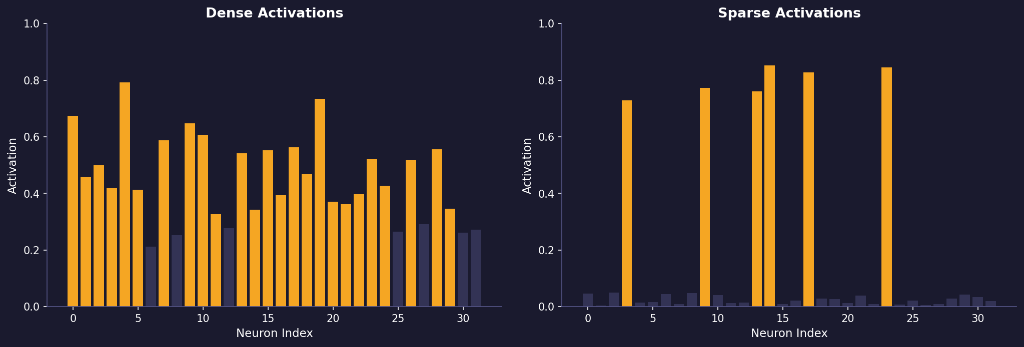
Let’s look at some typical activation patterns:
# Dense (standard) autoencoder activation example
# [0.6, 0.4, 0.5, 0.3, 0.7, 0.4, 0.6, 0.5]
# Many neurons are active simultaneously

# Sparse autoencoder activation example
# [0.01, 0.8, 0.02, 0.01, 0.03, 0.9, 0.02, 0.01]
# Only a few neurons are strongly active
Consider an image processing task:
# Example: Processing a 32x32 image patch
patch = load_image_patch(32, 32)  # 1024 dimensions

# Configure sparse autoencoder
encoder = SparseAutoencoder(
    input_dim=1024,
    hidden_dim=256,  # 4x compression
    rho=0.05,  # Expect 5% average activation
    beta=1.0
)

# Process the patch
reconstructed, hidden_repr, activations = encoder.forward(patch)

# Example hidden representation might look like:
# Most values near 0, with few strong activations:
# [0.01, 0.00, 0.87, 0.02, 0.00, 0.92, ...]
Implementation Tips
- Initialization: Initialize weights using a normal distribution with small variance (e.g., 0.01) to avoid saturation:
W = numpy.random.normal(0, 0.01, (input_dim, hidden_dim))- Monitoring: Track both reconstruction error and average activations:
def monitor_sparsity(hidden_activations):
    avg_activation = numpy.mean(hidden_activations)
    active_neurons = numpy.mean(hidden_activations > 0.1)
    print(f"Average activation: {avg_activation:.3f}")
print(f"Proportion of active neurons: {active_neurons:.3f}")- Hyperparameter Selection:
# Conservative starting points
hyperparams = {
    'learning_rate': 0.001,
    'rho': 0.05,        # Target sparsity
    'beta': 1.0,        # Sparsity weight
    'batch_size': 128,
    'hidden_dim': input_dim // 4  # 4x compression
}
The power of sparse autoencoders lies in their ability to discover specialized feature detectors. Each neuron becomes sensitive to specific patterns in the input data, making the learned representations more interpretable and often more useful for downstream tasks like classification or anomaly detection.
Remember that the sparsity constraint isn’t about having fewer neurons, but rather about having fewer neurons active at once. This mimics biological neural networks, where energy efficiency is achieved through sparse activation patterns.