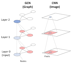
Graph Convolutional Networks

Graph Convolutional Networks extend deep learning to graph-structured data by generalizing the convolution operation from regular grids (like images) to irregular graph domains. The key innovation lies in how they aggregate and transform feature information from a node’s local neighborhood through spectral or spatial convolutions. In GCNs, each layer performs neighborhood feature aggregation where a node’s representation is updated by combining its features with those of its adjacent nodes. This aggregation is typically followed by a non-linear transformation. The process can be mathematically represented as a function of the normalized adjacency matrix, feature matrix, and learned weight matrices. Here’s the pseudocode for a basic GCN layer:
def GCN_layer(adjacency_matrix A, feature_matrix X, weight_matrix W):
    # Add self-loops to adjacency matrix
    A_hat = A + identity_matrix(A.shape[0])

    # Compute degree matrix
    D = diagonal_matrix([sum(row) for row in A_hat])

    # Symmetric normalization
    D_inv_sqrt = inverse_sqrt(D)
    A_norm = D_inv_sqrt @ A_hat @ D_inv_sqrt

    # Feature transformation and aggregation
    H = relu(A_norm @ X @ W)

    return H

def GCN_forward(G, X):
    # Initialize learnable weight matrices
    W1 = initialize_weights(input_dim, hidden_dim)
    W2 = initialize_weights(hidden_dim, output_dim)

    # First GCN layer
    H1 = GCN_layer(G.adjacency, X, W1)

    # Second GCN layer
    H2 = GCN_layer(G.adjacency, H1, W2)

    # Final node representations
    return H2
The core operation performs message passing through  = D(-1/2)(A + I)D(-1/2), where A is the adjacency matrix, I is the identity matrix (self-loops), and D is the degree matrix. This normalization prevents numerical instabilities and exploding/vanishing gradients. Each layer then applies this normalized adjacency matrix to the node features, followed by a learned weight transformation and non-linearity.