A comprehensive list of different types of VAEs Oct 13, 2024

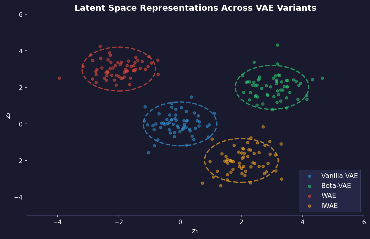
VAE (Vanilla VAE): The original VAE architecture consists of an encoder that maps input data to a latent space, and a decoder that reconstructs the input from the latent representation. It uses a variational inference approach to learn the latent space distribution.
Conditional VAE: This VAE variant incorporates additional conditioning information into both the encoder and decoder networks. The conditioning allows the model to generate samples conditioned on specific attributes or classes.
WAE - MMD (with RBF Kernel): Wasserstein Autoencoders use Maximum Mean Discrepancy (MMD) with a Radial Basis Function (RBF) kernel to minimize the distance between the encoded distribution and a prior distribution, aiming for better-quality reconstructions.
WAE - MMD (with IMQ Kernel): Similar to the RBF kernel version, but uses an Inverse MultiQuadric (IMQ) kernel for the MMD calculation, which can provide different regularization properties.
Beta-VAE: This architecture introduces a hyperparameter β to control the trade-off between reconstruction quality and the disentanglement of latent representations, allowing for more interpretable latent spaces.
Disentangled Beta-VAE: An improved version of Beta-VAE that aims to achieve better disentanglement of latent factors by modifying the training objective and architecture slightly.
Beta-TC-VAE: This variant decomposes the KL divergence term in the VAE objective into three components, with a β parameter applied to the total correlation term to encourage disentanglement.
IWAE (Importance Weighted Autoencoder): IWAE uses multiple samples from the encoder to compute a tighter lower bound on the marginal likelihood, potentially leading to better generative models.
MIWAE (Multiply Importance Weighted Autoencoder): An extension of IWAE that uses multiple importance-weighted samples during both training and inference to improve performance.
DFCVAE (Deep Feature Consistent VAE): This VAE incorporates perceptual losses based on features from pre-trained neural networks to improve the quality and consistency of generated images.
MSSIM VAE (Multi-Scale Structural Similarity VAE): This architecture uses a multi-scale structural similarity index as part of its loss function to improve the perceptual quality of reconstructed images.
Categorical VAE: A VAE variant designed to work with categorical latent variables, often using the Gumbel-Softmax trick for differentiable sampling from discrete distributions.
Joint VAE: This model combines continuous and discrete latent variables in a single framework, allowing for representation of both continuous and categorical factors.
Info VAE: InfoVAE modifies the objective function to maximize the mutual information between inputs and latent variables, aiming for more informative latent representations.
LogCosh VAE: This VAE uses the log-cosh loss function instead of mean squared error for reconstruction, potentially providing robustness to outliers.
SWAE (Sliced-Wasserstein Autoencoder): SWAE uses the sliced Wasserstein distance to measure the discrepancy between the encoded distribution and the prior, offering an alternative to KL divergence.
VQ-VAE (Vector Quantized VAE): This architecture uses vector quantization in the latent space, mapping continuous encodings to discrete codes from a codebook, useful for generating high-quality images and audio.
DIP VAE (Disentangled Inferred Prior VAE): DIP-VAE modifies the VAE objective to encourage the aggregate posterior to match the prior, aiming for better disentanglement of latent factors.

The math every variant above builds on #

Every model in this list modifies one object, the evidence lower bound (ELBO). So I think it is worth deriving it carefully once. Here is the setup. Data $x$ is generated from a latent $z$ by a decoder $p_\theta(x \mid z)$ with prior $p(z)$, usually $\mathcal{N}(0, I)$. The true posterior $p_\theta(z \mid x) = p_\theta(x \mid z)\, p(z)/p_\theta(x)$ is intractable, because the evidence $p_\theta(x) = \int p_\theta(x \mid z)\, p(z)\, dz$ is. So we introduce an encoder $q_\phi(z \mid x)$ that approximates it. Here $\theta$ are the decoder parameters and $\phi$ the encoder parameters.

The ELBO via the Jensen inequality #

Multiply and divide by $q_\phi$ inside the integral, then use the concavity of $\log$ (Jensen: $\log \mathbb{E}[Y] \ge \mathbb{E}[\log Y]$):

$$\begin{aligned} \log p_\theta(x) &= \log \int q_\phi(z \mid x)\, \frac{p_\theta(x, z)}{q_\phi(z \mid x)}\, dz = \log \mathbb{E}_{q_\phi(z \mid x)}\Big[\frac{p_\theta(x, z)}{q_\phi(z \mid x)}\Big] \\ &\ge \mathbb{E}_{q_\phi(z \mid x)}\Big[\log \frac{p_\theta(x, z)}{q_\phi(z \mid x)}\Big] =: \mathcal{L}(\theta, \phi; x). \end{aligned}$$

Splitting $p_\theta(x, z) = p_\theta(x \mid z)\, p(z)$ gives the familiar two-term form:

$$\mathcal{L}(\theta, \phi; x) = \underbrace{\mathbb{E}_{q_\phi(z \mid x)}\big[\log p_\theta(x \mid z)\big]}_{\text{reconstruction}} - \underbrace{D_{\mathrm{KL}}\big(q_\phi(z \mid x)\,\|\,p(z)\big)}_{\text{regularizer}}.$$

(IWAE in the list above tightens exactly this Jensen step. It averages $K$ importance weights inside the $\log$ before applying the inequality.)

The ELBO via the KL gap #

Jensen tells us that the bound holds but not how loose it is. The second derivation answers that. Because $\log p_\theta(x)$ does not depend on $z$, it equals its own expectation under $q_\phi$. Then use $p_\theta(x) = p_\theta(x, z)/p_\theta(z \mid x)$:

$$\log p_\theta(x) = \mathbb{E}_{q_\phi}\Big[\log \frac{p_\theta(x, z)}{p_\theta(z \mid x)}\Big] = \mathbb{E}_{q_\phi}\Big[\log \frac{p_\theta(x, z)}{q_\phi(z \mid x)}\Big] + \mathbb{E}_{q_\phi}\Big[\log \frac{q_\phi(z \mid x)}{p_\theta(z \mid x)}\Big],$$

that is,

$$\log p_\theta(x) = \mathcal{L}(\theta, \phi; x) + D_{\mathrm{KL}}\big(q_\phi(z \mid x)\,\|\,p_\theta(z \mid x)\big).$$

The gap is exactly the KL divergence from the encoder to the true posterior. Since it is non-negative, we recover the bound. Moreover, because $\log p_\theta(x)$ does not depend on $\phi$, maximizing $\mathcal{L}$ over $\phi$ is the same as minimizing that KL. One objective trains the decoder (push up the evidence) and turns the encoder into a better posterior approximation.

The reparameterization trick #

The reconstruction term is an expectation under a distribution that depends on $\phi$, so we cannot simply move $\nabla_\phi$ inside a Monte Carlo average. With a diagonal Gaussian encoder $q_\phi(z \mid x) = \mathcal{N}\big(z;\ \mu_\phi(x),\ \operatorname{diag}\sigma_\phi^2(x)\big)$, write the sample as a deterministic, differentiable function of parameter-free noise:

$$z = \mu_\phi(x) + \sigma_\phi(x) \odot \epsilon,\qquad \epsilon \sim \mathcal{N}(0, I),$$

where $\odot$ is element-wise multiplication. Now the randomness no longer depends on $\phi$, and the gradient passes through the sample:

$$\nabla_\phi\, \mathbb{E}_{q_\phi(z \mid x)}\big[f(z)\big] = \mathbb{E}_{\epsilon \sim \mathcal{N}(0, I)}\big[\nabla_\phi f\big(\mu_\phi(x) + \sigma_\phi(x) \odot \epsilon\big)\big].$$

A single sample of $\epsilon$ per data point already gives a low-variance, unbiased estimate. The alternative score-function (REINFORCE) estimator, $\mathbb{E}_{q_\phi}[f(z)\, \nabla_\phi \log q_\phi(z \mid x)]$, is also unbiased, but its variance is typically far higher. The Categorical VAE in the list needs the Gumbel-Softmax relaxation precisely because a discrete sample cannot be reparameterized this way.

The KL term in closed form #

With a diagonal Gaussian encoder and a standard normal prior, the regularizer needs no sampling. The KL factorizes over the $J$ latent dimensions, and for a single dimension, with $z \sim \mathcal{N}(\mu, \sigma^2)$,

$$\begin{aligned} D_{\mathrm{KL}}\big(\mathcal{N}(\mu, \sigma^2)\,\|\,\mathcal{N}(0, 1)\big) &= \mathbb{E}\Big[-\tfrac12\log(2\pi\sigma^2) - \frac{(z-\mu)^2}{2\sigma^2} + \tfrac12\log(2\pi) + \frac{z^2}{2}\Big] \\ &= -\tfrac12\log\sigma^2 - \tfrac12 + \tfrac12(\mu^2 + \sigma^2), \end{aligned}$$

using $\mathbb{E}[(z-\mu)^2] = \sigma^2$ and $\mathbb{E}[z^2] = \mu^2 + \sigma^2$. Summing over dimensions:

$$D_{\mathrm{KL}}\big(q_\phi(z \mid x)\,\|\,\mathcal{N}(0, I)\big) = \frac{1}{2}\sum_{j=1}^{J}\big(\mu_j^2 + \sigma_j^2 - \log\sigma_j^2 - 1\big).$$

Each summand is zero exactly when $\mu_j = 0$ and $\sigma_j = 1$. For the reconstruction term, a Gaussian decoder with fixed variance turns $-\log p_\theta(x \mid z)$ into a scaled squared error, and a Bernoulli decoder turns it into binary cross-entropy. That is why VAE code looks like “MSE + KL”.

$\beta$-VAE #

$\beta$-VAE puts a single weight $\beta$ on the regularizer:

$$\mathcal{L}_\beta(\theta, \phi; x) = \mathbb{E}_{q_\phi(z \mid x)}\big[\log p_\theta(x \mid z)\big] - \beta\, D_{\mathrm{KL}}\big(q_\phi(z \mid x)\,\|\,p(z)\big).$$

For $\beta = 1$ this is the ELBO. For $\beta > 1$ it is still a lower bound on $\log p_\theta(x)$, only looser, since the KL is non-negative. For $\beta < 1$ it is not a bound at all. To see what the extra pressure does, average the KL over the data distribution $p_{\text{data}}(x)$. Insert the aggregate posterior $q_\phi(z) = \mathbb{E}_{p_{\text{data}}(x)}[q_\phi(z \mid x)]$ into the log ratio:

$$\mathbb{E}_{p_{\text{data}}(x)}\Big[D_{\mathrm{KL}}\big(q_\phi(z \mid x)\,\|\,p(z)\big)\Big] = I_q(x; z) + D_{\mathrm{KL}}\big(q_\phi(z)\,\|\,p(z)\big),$$

where $I_q(x; z)$ is the mutual information between $x$ and $z$ under the encoder’s joint $p_{\text{data}}(x)\, q_\phi(z \mid x)$. Raising $\beta$ therefore does two things. It limits how much information the code carries about the input, which acts as a bottleneck. And it pushes the aggregate posterior towards the factorized prior, which is the pressure towards disentanglement. The price is blurrier reconstructions. Burgess et al. make the bottleneck explicit with a capacity target $C$ that is increased during training, $\mathbb{E}[\log p_\theta(x \mid z)] - \gamma\,\big|D_{\mathrm{KL}}(q_\phi(z \mid x)\,\|\,p(z)) - C\big|$. Beta-TC-VAE in the list goes one step further. It splits the $D_{\mathrm{KL}}(q_\phi(z)\,\|\,p(z))$ term again and penalizes only the total-correlation part.

References #

Diederik P. Kingma, Max Welling. Auto-Encoding Variational Bayes. ICLR 2014.
Danilo Jimenez Rezende, Shakir Mohamed, Daan Wierstra. Stochastic Backpropagation and Approximate Inference in Deep Generative Models. ICML 2014.
Christopher P. Burgess, Irina Higgins, Arka Pal, Loic Matthey, Nick Watters, Guillaume Desjardins, Alexander Lerchner. Understanding disentangling in β-VAE. 2018.

Related posts

Comments