Some common divergences
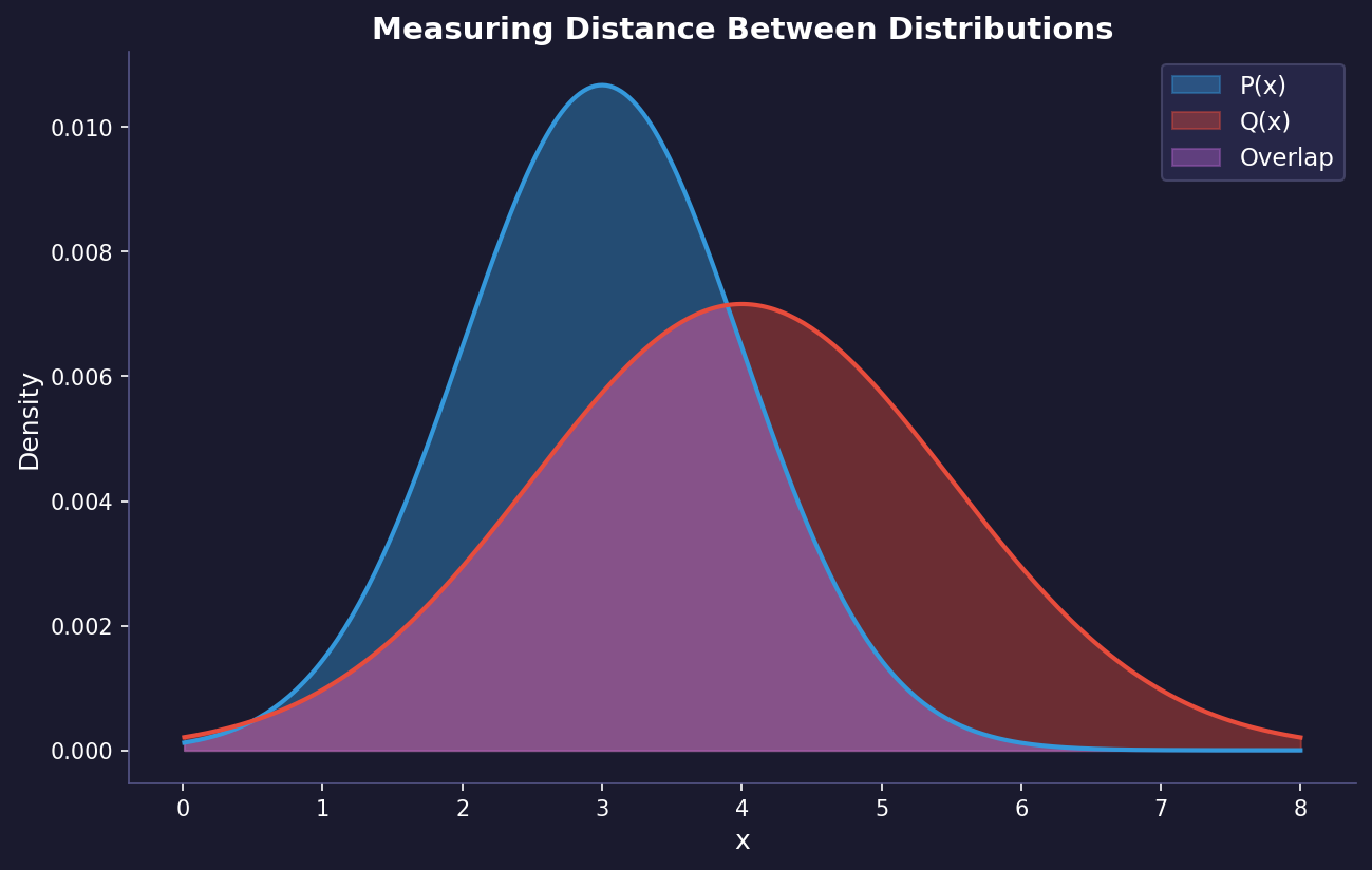
Hey. usually on machine learning we have to consider distances between different probability distributions. This is in fact a hard problem and there is a misconception that the most common way to do this is using the kl divergence. I believe that this is not true.
In fact, the KL divergence is not a metric, because it is not symmetric. It have nice properties that makes it useful but there are other metrics that are more useful in specific scenarios. Sadly these metrics are not taught on introductory courses in machine learning but there is a research trend on using these metrics on common architectures where you usually use the KL divergence on the loss, suck as the VAE’s and DDPMs.
The asymmetry is easier to believe when you can move the distributions around
yourself. Drag P and Q below: the two KL numbers are computed from the same
pair and they disagree, while the three symmetric measures underneath do not
care which distribution you call which. Try Same mean — two distributions
centred identically, one narrow and one wide — and watch KL(P‖Q) and
KL(Q‖P) differ by more than a nat. That gap is the whole reason the
mode-seeking and mass-covering behaviours of a VAE depend on which way round you
write the loss.
For example, here is code for some common divergences. The block below actually runs in your browser (Python via Pyodide, with NumPy): press Run, or Edit to try your own distributions.
import numpy as np
from scipy.spatial.distance import cosine, euclidean
from numpy.linalg import inv

def kl_divergence(p, q):
    """
    Compute the Kullback-Leibler divergence D_KL(P || Q)
    """
    p = np.asarray(p, dtype=np.float64)
    q = np.asarray(q, dtype=np.float64)
    epsilon = 1e-10
    p = np.clip(p, epsilon, 1)
    q = np.clip(q, epsilon, 1)
    return np.sum(p * np.log(p / q))

def js_divergence(p, q):
    """
    Compute the Jensen-Shannon divergence between distributions P and Q
    """
    m = 0.5 * (p + q)
    return 0.5 * kl_divergence(p, m) + 0.5 * kl_divergence(q, m)

def hellinger_distance(p, q):
    """
    Compute the Hellinger distance between distributions P and Q
    """
    return np.sqrt(np.sum((np.sqrt(p) - np.sqrt(q))**2)) / np.sqrt(2)

def total_variation_distance(p, q):
    """
    Compute the Total Variation distance between distributions P and Q
    """
    return 0.5 * np.sum(np.abs(p - q))

def bhattacharyya_distance(p, q):
    """
    Compute the Bhattacharyya distance between distributions P and Q
    """
    bc = np.sum(np.sqrt(p * q))
    return -np.log(bc)

def cosine_distance(p, q):
    """
    Compute the Cosine distance between distributions P and Q
    """
    return cosine(p, q)

def euclidean_distance(p, q):
    """
    Compute the Euclidean distance between distributions P and Q
    """
    return euclidean(p, q)

def chi_squared_distance(p, q):
    """
    Compute the Chi-Squared distance between distributions P and Q
    """
    epsilon = 1e-10
    p = np.asarray(p, dtype=np.float64) + epsilon
    q = np.asarray(q, dtype=np.float64) + epsilon
    return 0.5 * np.sum(((p - q)**2) / (p + q))

def kolmogorov_smirnov_statistic(p, q):
    """
    Compute the Kolmogorov-Smirnov statistic between distributions P and Q
    """
    cdf_p = np.cumsum(p)
    cdf_q = np.cumsum(q)
    return np.max(np.abs(cdf_p - cdf_q))

def mahalanobis_distance(p, q, cov=None):
    """
    Compute the Mahalanobis distance between distributions P and Q
    """
    diff = p - q
    if cov is None:
        cov = np.cov(np.stack([p, q], axis=0).T)
    cov_inv = inv(cov)
    return np.sqrt(np.dot(np.dot(diff.T, cov_inv), diff))

p = np.array([0.1, 0.2, 0.3, 0.4])
q = np.array([0.4, 0.3, 0.2, 0.1])

for name, f in [("KL(P||Q)", kl_divergence), ("KL(Q||P)", lambda a, b: kl_divergence(b, a)),
                ("Jensen-Shannon", js_divergence), ("Hellinger", hellinger_distance),
                ("Total variation", total_variation_distance),
                ("Bhattacharyya", bhattacharyya_distance), ("Cosine", cosine_distance),
                ("Euclidean", euclidean_distance),
                ("Chi-squared", chi_squared_distance), ("KS statistic", kolmogorov_smirnov_statistic)]:
print(f"{name:16s} {f(p, q):.4f}")One family behind most of these: f-divergences #
Most of the functions above look like unrelated formulas, but KL in both directions, Jensen-Shannon, total variation, Hellinger and $\chi^2$ are all the same object with a different convex function plugged in.
Definition #
Let $P$ and $Q$ be distributions with densities (or probability mass functions) $p$ and $q$, and assume $P$ is absolutely continuous with respect to $Q$: $q(x) = 0$ implies $p(x) = 0$. Let $f : (0, \infty) \to \mathbb{R}$ be convex with $f(1) = 0$. The $f$-divergence is
$$D_f(P \,\|\, Q) = \mathbb{E}_{x \sim Q}\!\left[ f\!\left(\frac{p(x)}{q(x)}\right) \right] = \int q(x)\, f\!\left(\frac{p(x)}{q(x)}\right) dx .$$
It measures how far the likelihood ratio $p/q$ is from $1$, averaged under $Q$ and weighted by how much $f$ penalises each deviation.
The usual suspects as instances #
| Divergence | $f(t)$ | $D_f(P \,\|\, Q)$ |
|---|---|---|
| KL | $t \log t$ | $\int p \log \frac{p}{q}$ |
| Reverse KL | $-\log t$ | $\int q \log \frac{q}{p}$ |
| Pearson $\chi^2$ | $(t-1)^2$ | $\int \frac{(p - q)^2}{q}$ |
| Total variation | $\frac{1}{2}\lvert t - 1\rvert$ | $\frac{1}{2}\int \lvert p - q \rvert$ |
| Squared Hellinger | $\frac{1}{2}(\sqrt{t} - 1)^2$ | $\frac{1}{2}\int (\sqrt{p} - \sqrt{q})^2$ |
| Jensen-Shannon | $\frac{1}{2}\left[t \log t - (1 + t)\log\frac{1+t}{2}\right]$ | $\frac{1}{2}\mathrm{KL}(P \,\|\, M) + \frac{1}{2}\mathrm{KL}(Q \,\|\, M)$ |
In the last row $M = \frac{1}{2}(P + Q)$. To check it, multiply $f(p/q)$ by $q$:
$\frac{1}{2}\left[p \log\frac{p}{q} - (p+q)\log\frac{p+q}{2q}\right] = \frac{1}{2}\left[p\log\frac{p}{m} + q \log\frac{q}{m}\right]$
with $m = \frac{1}{2}(p+q)$. The Hellinger normalisation matches
hellinger_distance in the code, which returns the square root of this
quantity. Note that chi_squared_distance above is the symmetric chi-squared
$\frac{1}{2}\sum (p-q)^2/(p+q)$, a cousin of Pearson’s $\chi^2$ and not the same
number. Two more facts: swapping $P$ and $Q$ corresponds to using
$t f(1/t)$ in place of $f(t)$, so a divergence is symmetric when the two agree
(TV, Hellinger and JS do). And adding $c(t-1)$ to $f$ never changes $D_f$,
because $\mathbb{E}_Q[p/q - 1] = 0$.
Non-negativity, from Jensen #
Since $f$ is convex, Jensen’s inequality gives
$$D_f(P \,\|\, Q) = \mathbb{E}_Q\!\left[f\!\left(\frac{p}{q}\right)\right] \ge f\!\left(\mathbb{E}_Q\!\left[\frac{p}{q}\right]\right) = f\!\left(\int q \frac{p}{q}\right) = f(1) = 0 .$$
If $f$ is strictly convex at $1$, equality holds only when $p/q$ is constant $Q$-almost everywhere, i.e. $P = Q$. So every member of the family is a valid “divergence”: non-negative and zero exactly at equality. None of them needs to be symmetric or satisfy the triangle inequality, which is my point about KL not being a metric. (TV and the square root of Hellinger are true metrics. So is the square root of JS.)
Forward vs reverse KL: covering vs seeking modes #
This is the gap you saw in the widget. Suppose $P$ is the data distribution and $Q_\theta$ is a model we fit by minimising a KL.
Forward KL, $\mathrm{KL}(P \,\|\, Q_\theta) = \mathbb{E}_P[\log p - \log q_\theta]$. The expectation is under $P$, so the cost blows up wherever $p(x) > 0$ but $q_\theta(x) \to 0$. The model is forced to put mass everywhere the data lives. If $P$ is bimodal and $Q_\theta$ is a single Gaussian, the optimum stretches across both modes and puts a lot of mass in the empty valley between them. This is mass-covering (or mean-seeking). Maximum likelihood is exactly this direction, since $\mathrm{KL}(P\,\|\,Q_\theta) = -\mathbb{E}_P[\log q_\theta] + \text{const}$.
Reverse KL, $\mathrm{KL}(Q_\theta \,\|\, P) = \mathbb{E}_{Q_\theta}[\log q_\theta - \log p]$. Now the expectation is under the model. Putting mass where $p \approx 0$ is very expensive, while ignoring a region where $p > 0$ costs nothing. The same single Gaussian now locks onto one mode and ignores the other. This is mode-seeking. Variational inference uses this direction: the gap in the ELBO of a VAE is $\mathrm{KL}(q_\phi(z \mid x) \,\|\, p(z \mid x))$. That is one reason variational posteriors tend to underestimate uncertainty.
The variational representation, and f-GAN #
Neither direction can be computed directly when all we have are samples from $P$ and $Q$, because we never get to evaluate $p/q$. The trick is convex duality. The Fenchel conjugate of $f$ is $f^*(u) = \sup_{t} \{ u t - f(t) \}$. For convex, lower semicontinuous $f$ we have $f = f^{**}$, i.e. $f(t) = \sup_u \{ u t - f^*(u) \}$. Plug that into the definition. Taking the supremum pointwise in $x$ with a function $T(x)$ in place of $u$, and noting that any particular $T$ gives a lower bound:
$$D_f(P \,\|\, Q) = \int q(x) \sup_{u}\left\{ u \frac{p(x)}{q(x)} - f^*(u) \right\} dx \;\ge\; \sup_{T} \Big( \mathbb{E}_{x \sim P}[T(x)] - \mathbb{E}_{x \sim Q}[f^*(T(x))] \Big).$$
The supremum is over functions $T$ from the sample space to the domain of $f^*$. The bound is tight, with $T^*(x) = f'\big(p(x)/q(x)\big)$, when the function class is rich enough. Both expectations on the right need only samples. For KL, $f(t) = t\log t$ gives $f^*(u) = e^{u-1}$, so
$$\mathrm{KL}(P \,\|\, Q) = \sup_T \; \mathbb{E}_P[T] - \mathbb{E}_Q\big[e^{T - 1}\big],$$
which is the Nguyen-Wainwright-Jordan estimator. f-GAN turns the bound into a game. A generator $Q_\theta$ and a critic $T_\omega$ play
$$\min_\theta \max_\omega \; \mathbb{E}_{x \sim P}[T_\omega(x)] - \mathbb{E}_{x \sim Q_\theta}[f^*(T_\omega(x))] .$$
The critic tightens the lower bound on $D_f$, and the generator pushes it down. Choosing $f$ picks the divergence the GAN minimises. The original GAN objective is the case $f(t) = t\log t - (1+t)\log(1+t)$, which equals $2\,\mathrm{JS}(P\,\|\,Q) - \log 4$.
Anyway, for more details here is the colab where I implemented some of these metrics and more Link to code
References #
-
-
- Ali, S. D. Silvey (1966). A General Class of Coefficients of Divergence of One Distribution from Another. Journal of the Royal Statistical Society, Series B 28(1), 131–142.
-
-
- Csiszár (1967). Information-type measures of difference of probability distributions and indirect observations. Studia Scientiarum Mathematicarum Hungarica 2, 299–318.
-
- Minka (2005). Divergence measures and message passing. Microsoft Research Technical Report MSR-TR-2005-173.
-
- Nguyen, M. J. Wainwright, M. I. Jordan (2010). Estimating divergence functionals and the likelihood ratio by convex risk minimization. IEEE Transactions on Information Theory 56(11). arXiv:0809.0853
-
- Nowozin, B. Cseke, R. Tomioka (2016). f-GAN: Training Generative Neural Samplers using Variational Divergence Minimization. NeurIPS. arXiv:1606.00709
Comments