Diffusion models or Autoencoders?
Unmasking the Secret Link: Are Diffusion Models Just Fancy Autoencoders? #
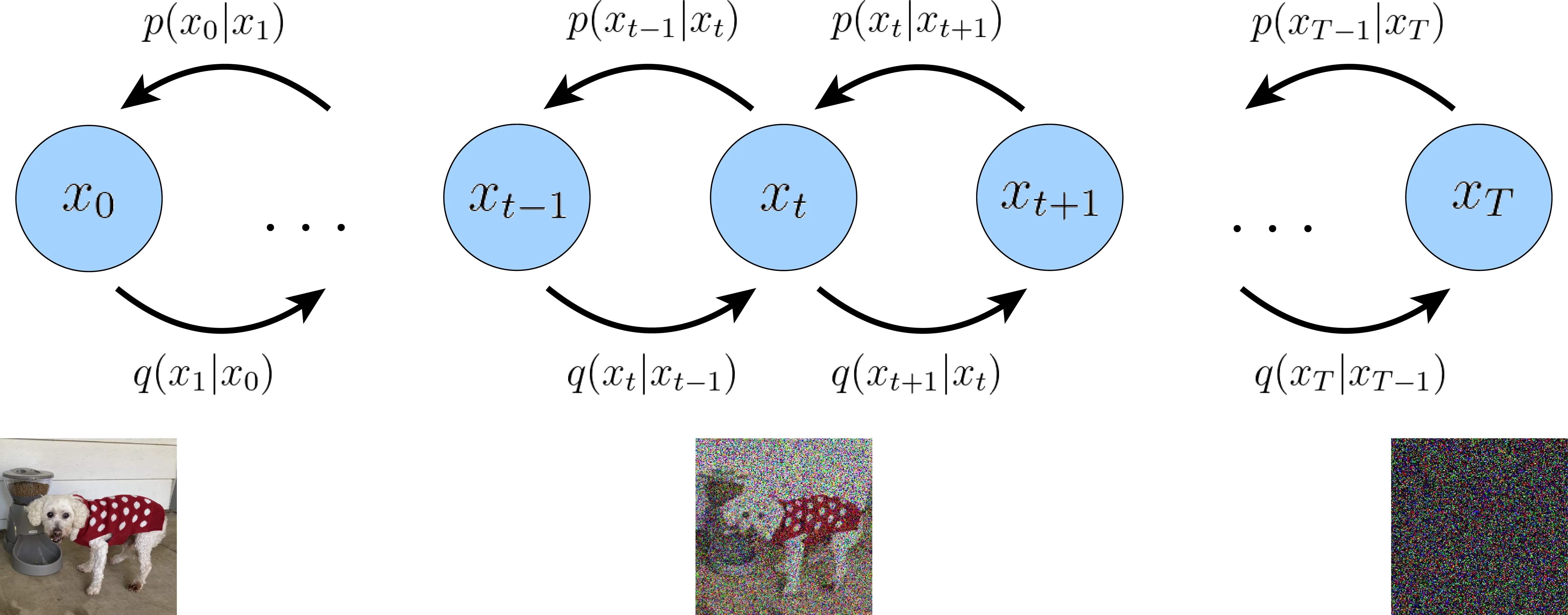
Recent advancements in generative AI have brought diffusion models to the forefront, particularly for their impressive performance in image generation. While these models are often seen as distinct from traditional approaches, there’s a compelling argument for viewing diffusion models as a form of hierarchical autoencoder.
The key insight lies in the similarity between the noise addition process in diffusion models and the compression step in autoencoders. When a diffusion model adds noise to data, it’s effectively compressing the information, retaining only the most robust features. This is analogous to how an autoencoder’s encoder compresses input data into a lower-dimensional representation.
Conversely, the denoising process in diffusion models resembles the reconstruction phase of autoencoders. The critical difference is that diffusion models perform this reconstruction gradually, over multiple steps, allowing them to capture a hierarchy of details. This multi-step process creates a series of latent representations at different levels of abstraction, much like a hierarchical autoencoder.
The noise in diffusion models serves a similar purpose to the bottleneck layer in autoencoders, acting as an information constraint that forces the model to learn efficient, robust representations. This perspective suggests that diffusion models implicitly learn a series of nested representations, each corresponding to a different noise level.
That is the argument in words. In this post I want to make it precise, because every sentence above has an exact mathematical counterpart, and a couple of them need a caveat once you write the math down. The plan:
- The forward process is an encoder, and it has a closed form.
- The diffusion training objective is literally the ELBO of a hierarchical VAE whose encoder is fixed. Each timestep contributes one KL term.
- Written in terms of the signal-to-noise ratio, that ELBO becomes a weighted denoising loss, and the popular “simple” loss is the same thing with a different weighting.
- Each term is a denoising autoencoder, and by Tweedie’s formula the optimal denoiser is the score. This is the link Vincent made in 2011, long before diffusion models.
- The “bottleneck” is a Gaussian channel whose capacity is set by the noise level, and it destroys fine detail before coarse structure. This is the precise sense in which noise “retains only the most robust features”, and it is the rate-distortion reading in Section 4.3 of Ho et al. (2020).
1. The forward process is a fixed encoder #
A DDPM (Sohl-Dickstein et al., 2015; Ho et al., 2020) defines a Markov chain that slowly adds Gaussian noise to a data point $x_0$:
$$q(x_t \mid x_{t-1}) = \mathcal{N}\big(x_t;\ \sqrt{\alpha_t}\, x_{t-1},\ \beta_t I\big), \qquad \alpha_t = 1 - \beta_t,\qquad t = 1, \dots, T.$$
The scaling by $\sqrt{\alpha_t}$ is what keeps the variance from blowing up. Because a linear map of a Gaussian plus independent Gaussian noise is Gaussian, the steps compose. Write $x_t = \sqrt{\alpha_t}\, x_{t-1} + \sqrt{1 - \alpha_t}\, \epsilon_t$ and suppose, by induction, that $x_{t-1} = \sqrt{\bar\alpha_{t-1}}\, x_0 + \sqrt{1 - \bar\alpha_{t-1}}\, \bar\epsilon$. Then $x_t$ is $\sqrt{\alpha_t \bar\alpha_{t-1}}\, x_0$ plus zero-mean Gaussian noise of variance $\alpha_t (1 - \bar\alpha_{t-1}) + (1 - \alpha_t) = 1 - \alpha_t\bar\alpha_{t-1}$. With $\bar\alpha_t = \prod_{s=1}^t \alpha_s$:
$$\begin{aligned} q(x_t \mid x_0) &= \mathcal{N}\big(x_t;\ \sqrt{\bar\alpha_t}\, x_0,\ (1 - \bar\alpha_t) I\big), \\ \text{i.e.}\quad x_t &= \sqrt{\bar\alpha_t}\, x_0 + \sqrt{1 - \bar\alpha_t}\, \epsilon,\quad \epsilon \sim \mathcal{N}(0, I). \end{aligned}$$
So the “encoder” maps $x_0$ to a whole family of codes $x_1, \dots, x_T$, and any one of them can be sampled in a single step. The schedule is chosen so that $\bar\alpha_T \approx 0$, which makes $q(x_T \mid x_0) \approx \mathcal{N}(0, I)$ regardless of $x_0$: the last code carries essentially no information about the input.
Two facts are worth stating now because they are where the analogy with a normal autoencoder bends. The encoder has no learnable parameters. And every code $x_t$ has the same dimension as $x_0$. There is no narrow layer anywhere. Whatever bottleneck exists has to come from the noise, and section 5 measures exactly how much.
2. The ELBO: a hierarchical VAE with a fixed encoder #
Recall the VAE bound. For a latent-variable model $p_\theta(x, z)$ and any encoder $q(z \mid x)$,
$$-\log p_\theta(x) \le \mathbb{E}_{q(z \mid x)}\left[ -\log \frac{p_\theta(x, z)}{q(z \mid x)} \right].$$
A hierarchical VAE has a stack of latents $z_1, \dots, z_T$ with a top-down decoder. Now take the latents to be $x_1, \dots, x_T$, the decoder to be a Markov chain running backwards,
$$p_\theta(x_{0:T}) = p(x_T) \prod_{t=1}^T p_\theta(x_{t-1} \mid x_t), \qquad p(x_T) = \mathcal{N}(0, I),$$
and the encoder to be the forward process $q(x_{1:T} \mid x_0) = \prod_t q(x_t \mid x_{t-1})$. Plug them into the bound. The trick that makes it tractable is to rewrite each encoder step using Bayes’ rule, conditioning on $x_0$ (which changes nothing, by the Markov property):
$$q(x_t \mid x_{t-1}) = q(x_t \mid x_{t-1}, x_0) = \frac{q(x_{t-1} \mid x_t, x_0)\, q(x_t \mid x_0)}{q(x_{t-1} \mid x_0)} .$$
The ratio $q(x_t \mid x_0)/q(x_{t-1} \mid x_0)$ telescopes across the product, and the bound splits into one term per level (Luo, 2022, walks through every line of this derivation):
$$\begin{aligned} -\log p_\theta(x_0) \le\ & \underbrace{\mathrm{KL}\big(q(x_T \mid x_0)\,\|\,p(x_T)\big)}_{L_T} \\ &+ \sum_{t=2}^{T} \underbrace{\mathbb{E}_{q}\, \mathrm{KL}\big(q(x_{t-1} \mid x_t, x_0)\,\|\,p_\theta(x_{t-1} \mid x_t)\big)}_{L_{t-1}} \\ &\underbrace{-\ \mathbb{E}_{q} \log p_\theta(x_0 \mid x_1)}_{L_0}. \end{aligned}$$
Read it as a VAE practitioner would:
- $L_0$ is the reconstruction term: decode $x_0$ from the least noisy code.
- $L_T$ is the prior term at the top of the hierarchy. It has no parameters and is approximately zero by design.
- Each $L_{t-1}$ is the KL term of one layer of the hierarchy: how well the decoder’s layer $t \to t-1$ matches the encoder’s posterior for that layer.
Every distribution in a KL term is Gaussian. The encoder posterior is available in closed form, because both $q(x_t \mid x_0)$ and $q(x_t \mid x_{t-1})$ are:
$$\begin{aligned} q(x_{t-1} \mid x_t, x_0) &= \mathcal{N}\big(\tilde\mu_t(x_t, x_0),\ \tilde\beta_t I\big), \\ \tilde\mu_t &= \frac{\sqrt{\bar\alpha_{t-1}}\,\beta_t}{1 - \bar\alpha_t}\, x_0 + \frac{\sqrt{\alpha_t}\,(1 - \bar\alpha_{t-1})}{1 - \bar\alpha_t}\, x_t, \\ \tilde\beta_t &= \frac{1 - \bar\alpha_{t-1}}{1 - \bar\alpha_t}\,\beta_t . \end{aligned}$$
The decoder only has to supply its guess of $x_0$. Give $p_\theta(x_{t-1} \mid x_t)$ the same variance $\tilde\beta_t$ and the same mean formula, with $x_0$ replaced by a network’s estimate $\hat x_\theta(x_t, t)$. A KL between two Gaussians with equal covariance is a squared distance between their means, so
$$L_{t-1} = \frac{1}{2\tilde\beta_t}\, \frac{\bar\alpha_{t-1}\beta_t^2}{(1 - \bar\alpha_t)^2}\; \mathbb{E}\,\big\| x_0 - \hat x_\theta(x_t, t) \big\|^2 .$$
So the diffusion model really is a hierarchical VAE, in the strict sense that its loss is a hierarchical VAE’s ELBO. What makes it special is the list of things it gives up and gets in return:
- Fixed encoder. In a learned hierarchical VAE the encoder and decoder co-adapt, and a well-known failure is that the KL terms push upper layers to carry no information at all (posterior collapse). Here the encoder cannot be optimised away from informative codes: every $x_t$ with $t < T$ contains information about $x_0$ by construction.
- Shared decoder. All $T$ layers of the decoder are one network, told which layer it is via $t$.
- Every layer is a regression problem. Each KL term reduces to a weighted mean-squared error, with no sampling of the encoder needed beyond a single draw of $x_t$.
- No dimensionality reduction. The price of the fixed encoder: the “compression” has to be done entirely by noise.
3. The signal-to-noise ratio, and the loss weighting #
The awkward-looking coefficient in $L_{t-1}$ has a clean form. Define the signal-to-noise ratio of the code at level $t$,
$$\mathrm{SNR}(t) = \frac{\bar\alpha_t}{1 - \bar\alpha_t},$$
the ratio of the variance of the signal part $\sqrt{\bar\alpha_t}\, x_0$ (per unit of data variance) to the variance of the noise. It decreases monotonically from very large at $t = 1$ to almost zero at $t = T$. Substituting $\tilde\beta_t$ and simplifying (the numerator $\bar\alpha_{t-1}(1 - \bar\alpha_t) - \bar\alpha_t(1 - \bar\alpha_{t-1})$ collapses to $\bar\alpha_{t-1} \beta_t$) gives the result of Kingma et al. (2021):
$$L_{t-1} = \tfrac{1}{2}\big( \mathrm{SNR}(t-1) - \mathrm{SNR}(t) \big)\; \mathbb{E}\,\big\| x_0 - \hat x_\theta(x_t, t) \big\|^2 .$$
Each layer of the hierarchy is a reconstruction error, weighted by how much SNR is lost between that layer and the one below. Take the continuous-time limit, write $\sigma_t = \sqrt{1 - \bar\alpha_t}$ for the noise scale, and parametrise by noise prediction, $\hat x_\theta = (x_t - \sigma_t \hat\epsilon_\theta)/\sqrt{\bar\alpha_t}$, so that $\|x_0 - \hat x_\theta\|^2 = \|\epsilon - \hat\epsilon_\theta\|^2 / \mathrm{SNR}(t)$. With $\lambda = \log \mathrm{SNR}$, the sum becomes an integral and the SNR factors cancel:
$$\mathcal{L}_{\text{ELBO}} = \tfrac{1}{2}\, \mathbb{E}_{x_0, \epsilon} \int_{\lambda_{\min}}^{\lambda_{\max}} \big\| \epsilon - \hat\epsilon_\theta(x_\lambda, \lambda) \big\|^2 \, d\lambda .$$
This is a striking statement. The ELBO is a denoising loss integrated uniformly in log-SNR. The schedule, i.e. how fast $t$ moves through log-SNR, does not appear at all: only the two endpoints do. Kingma et al. make exactly this point: in continuous time the bound is invariant to the noise schedule except at its endpoints. The schedule only changes the variance of the Monte Carlo estimate of the integral.
Ho et al. did not train on the ELBO. They found better samples with the “simple” loss $\mathbb{E}_{t \sim \mathcal{U}}\, \|\epsilon - \hat\epsilon_\theta\|^2$, which samples $t$ uniformly. A change of variables shows that this is the same integral with a weight: if $t$ is uniform on $[0, 1]$ then $\lambda$ has some density $p(\lambda)$, and
$$\mathcal{L}_{\text{simple}} = \int p(\lambda)\; \mathbb{E}\,\big\| \epsilon - \hat\epsilon_\theta(x_\lambda, \lambda) \big\|^2 \, d\lambda , \qquad\text{a weighted ELBO with } w(\lambda) \propto p(\lambda).$$
For the cosine schedule of Nichol and Dhariwal (2021), $\bar\alpha_t = \cos^2(\pi t/2)$ (ignoring their small offset), one gets $\lambda = -2\log\tan(\pi t/2)$ and $p(\lambda) = \tfrac{1}{2\pi}\operatorname{sech}(\lambda/2)$: a bump centred at SNR = 1 that down-weights both very clean and very noisy levels relative to the ELBO. In other words, choosing a loss weighting is choosing which layers of the hierarchical autoencoder to care about. The ELBO cares about all of them equally in log-SNR, including the almost-clean levels that only encode imperceptible detail (we will see in section 5 that this is where most of the bits go). Perceptual quality prefers to spend capacity in the middle.
Kingma and Gao (2023) close the loop: when the weighting $w(\lambda)$ is monotone in the noise level, the weighted loss equals the ELBO of the data augmented with Gaussian noise perturbations. The sech weighting above is not monotone, so it does not fall under that result as stated. They then report state-of-the-art FID with new monotone weightings.
4. Every layer is a denoising autoencoder #
So far $\hat x_\theta$ was just “the decoder’s guess of $x_0$”. What is the best possible guess? The loss at each level is a mean-squared error, so the minimiser is the posterior mean $\mathbb{E}[x_0 \mid x_t]$. And for Gaussian corruption the posterior mean has a remarkable closed form, Tweedie’s formula (see Efron, 2011). If $z = \alpha x + \sigma \epsilon$ then
$$\mathbb{E}[x \mid z] = \frac{z + \sigma^2 \nabla_z \log p(z)}{\alpha} .$$
The proof is one line. Differentiate $p(z) = \int p(x)\, \mathcal{N}(z; \alpha x, \sigma^2 I)\, dx$ under the integral: $\nabla_z p(z) = \int p(x)\, \mathcal{N}(z; \alpha x, \sigma^2 I)\, \frac{\alpha x - z}{\sigma^2}\, dx$. Divide by $p(z)$ and the right side becomes $(\alpha\, \mathbb{E}[x \mid z] - z)/\sigma^2$.
Two consequences:
- The optimal denoiser is the score. Learning to denoise at noise level $t$ is the same as learning $\nabla \log p_t(x_t)$, the score of the noised data distribution. In noise-prediction form, $\hat\epsilon^*(x_t) = -\sigma_t \nabla \log p_t(x_t)$.
- The diffusion loss is denoising score matching. Vincent (2011) showed that training a model $s_\theta(\tilde x)$ to match $\nabla_{\tilde x} \log q_\sigma(\tilde x \mid x) = -(\tilde x - x)/\sigma^2$, the score of the corruption kernel, is equivalent up to a constant to matching the score of the corrupted data distribution $q_\sigma(\tilde x)$, and that this is what a denoising autoencoder with Gaussian noise is doing. With $\tilde x - x \propto \epsilon$, that is exactly the $\epsilon$-prediction loss. Song and Ermon (2019) built a generative model directly on this, with Langevin dynamics over a ladder of noise levels; Song et al. (2020) unified both views as a stochastic differential equation.
So the precise version of “the denoising process resembles the reconstruction phase of autoencoders” is: a diffusion model is a stack of denoising autoencoders, one per noise level, with tied weights, trained with the weights given by the ELBO (or a reweighting of it), and chained together at sampling time. The autoencoder at level $t$ is a DAE in Vincent’s sense; the chain is what turns a family of DAEs into a generative model.
There is one place where the autoencoder intuition is misleading, and it matters. At high noise the optimal reconstruction $\mathbb{E}[x_0 \mid x_t]$ is a blurry average of all the images consistent with $x_t$, not an image. A one-shot autoencoder at that level would be bad. The sampler never uses it that way: it takes a small step toward the posterior mean, re-noises, and asks again. The detail that the encoder destroyed is not reconstructed; it is sampled, consistently with whatever coarse structure survived.
5. What the noise destroys: a bottleneck with a known capacity #
Now the claim that noise acts like a bottleneck. The code $x_t = \sqrt{\bar\alpha_t}\, x_0 + \sqrt{1-\bar\alpha_t}\,\epsilon$ is the output of an additive Gaussian noise channel. If $x_0$ has covariance $\Sigma$ with eigenvalues $\lambda_k$, the information the code carries is bounded by the Gaussian channel capacity,
$$I(x_0; x_t) \;\le\; \tfrac{1}{2}\log\det\big(I + \mathrm{SNR}(t)\, \Sigma\big) = \sum_k \tfrac{1}{2}\log\big(1 + \mathrm{SNR}(t)\, \lambda_k\big),$$
with equality when $x_0$ is Gaussian (a Gaussian has the largest entropy for a given covariance). Two things follow.
The noise level sets the size of the bottleneck. Unlike a narrow layer, which caps the information at “number of units times bits per unit”, the cap here is continuous and controlled by a single number, $\mathrm{SNR}(t)$. Sweeping $t$ sweeps the bottleneck from “almost everything” to “nothing”.
It removes low-variance directions first. A direction with $\mathrm{SNR}(t)\,\lambda_k \gg 1$ is barely affected, while one with $\mathrm{SNR}(t)\,\lambda_k \ll 1$ is essentially erased. For natural images the variance is concentrated in low spatial frequencies (the power spectrum falls off roughly like a power of frequency), so as $t$ grows the noise drowns the fine details first and the coarse layout last. Generation runs this backwards: coarse to fine. Dieleman (2024) makes the striking observation that this makes image diffusion an approximate autoregression in frequency space.
There is a nice rate-distortion way to say this. For a Gaussian component of variance $\lambda$, the best estimator from $x_t$ has error $D = \lambda / (1 + \mathrm{SNR}\cdot\lambda)$ and the channel carries $R = \tfrac{1}{2}\log(1 + \mathrm{SNR}\cdot\lambda) = \tfrac{1}{2}\log(\lambda/D)$ nats, which is exactly the Gaussian rate-distortion function. So every component, on its own, sits on the optimal rate-distortion curve. Across components the allocation is a soft version of reverse water-filling: strong components end up with distortion close to $1/\mathrm{SNR}$ (the “water level”), and weak ones are dropped almost entirely, with distortion close to their full variance. That is, in my reading, the cleanest formal sense in which “adding noise is compressing, keeping the robust features”.
Ho et al. (2020, Section 4.3) measure this on real images. They treat the KL terms $L_1 + \dots + L_T$ as the rate and $L_0$ as the distortion, and set up a progressive lossy code: send $x_T, x_{T-1}, \dots$ one after another, with the receiver predicting $\hat x_0$ from whatever $x_t$ it has so far. Three findings:
- Their best CIFAR-10 model has a rate of 1.78 bits/dim and a distortion of 1.97 bits/dim (RMSE 0.95 on a 0 to 255 scale). In their words, more than half of the lossless codelength describes imperceptible distortions.
- In the rate-distortion curve, the distortion falls steeply over the first small fraction of the rate. The first few bits buy almost all of the perceptual content.
- Samples from $p_\theta(x_0 \mid x_t)$ with $x_t$ held fixed share large-scale attributes and differ in details: when $t$ is large, only large-scale features are preserved. They call it, carefully, a hint of conceptual compression.
You can also see why the curve looks like that. With an ideal reverse model, the expected KL for the step $t \to t-1$ is $I(x_0; x_{t-1} \mid x_t) = I(x_0; x_{t-1}) - I(x_0; x_t)$ (chain rule plus the Markov property of the forward process), so the rate accumulated by the time the receiver holds $x_t$ telescopes to exactly $I(x_0; x_t)$, the quantity bounded above. Rate in this code is the mutual information between the data and the current code.
This backs up the original claim that the view “hints at applications beyond generation, such as in data compression”. The caveat is practical, not conceptual: Ho et al.’s scheme assumes a procedure (such as minimal random coding) that can transmit a sample from $q$ using about $\mathrm{KL}(q \,\|\, p)$ bits, and such procedures are expensive in high dimension. It is a statement about what the model could compress, not a codec you can ship.
Try it #
The block below runs in your browser (Python via Pyodide, with NumPy). It uses a toy “image”: a Gaussian signal of length 256 whose Fourier coefficients have variance proportional to $1/f^2$, roughly the falloff of natural images. Because the prior is Gaussian, everything is in closed form: the mutual information each frequency band keeps at each $t$, and the error of the best possible denoiser. It then checks the closed form by building that denoiser from the score with Tweedie’s formula and measuring its error by Monte Carlo, and it prints the “equal-power frequency”, where signal and noise have the same variance, as $t$ grows.
import numpy as np

rng = np.random.default_rng(0)

# A toy "image": a 1-D Gaussian signal of length D whose Fourier coefficients
# have variance ~ 1/f^2, the power law natural images roughly follow.
# In that basis x0 has a diagonal covariance, so everything is closed form.
D = 256
f = np.arange(1, D + 1)              # frequency index of each coefficient
lam = 1.0 / f**2
lam *= D / lam.sum()                 # normalise: total variance D (unit per pixel)

# Cosine schedule (Nichol & Dhariwal style), T = 1000 steps
T = 1000
s = 0.008
abar = np.cos((np.arange(T + 1) / T + s) / (1 + s) * np.pi / 2) ** 2
abar = np.clip(abar / abar[0], 1e-8, 1.0)
snr = abar / (1 - abar + 1e-12)

def mi_per_coeff(t):
    # I(x0_k ; x_t_k) = 1/2 log(1 + SNR(t) * lam_k)   (Gaussian channel)
    return 0.5 * np.log1p(snr[t] * lam)

def mmse_per_coeff(t):
    # E[(x0_k - E[x0_k | x_t])^2] = lam_k / (1 + SNR(t) * lam_k)
    return lam / (1 + snr[t] * lam)

bands = {"coarse f<=4": f <= 4, "mid 4<f<=32": (f > 4) & (f <= 32), "fine f>32": f > 32}

print("Information about x0 that survives in x_t (nats), by frequency band,")
print("and the relative error of the best possible denoiser E[x0 | x_t].\n")
print(f"{'t':>5} {'log SNR':>8} " + " ".join(f"{b:>12}" for b in bands) + f" {'total':>8} {'rel. MSE':>9}")
for t in [1, 50, 150, 300, 500, 700, 850, 950, 1000]:
    mi = mi_per_coeff(t)
    rel = mmse_per_coeff(t).sum() / lam.sum()
    cols = " ".join(f"{mi[m].sum():12.2f}" for m in bands.values())
    print(f"{t:5d} {np.log(snr[t]):8.2f} {cols} {mi.sum():8.2f} {rel:9.3f}")

print("\nFraction of each band's variance the best denoiser recovers from x_t:\n")
print(f"{'t':>5} " + " ".join(f"{b:>12}" for b in bands))
for t in [50, 150, 300, 500, 700, 850, 950]:
    r2 = 1 - mmse_per_coeff(t) / lam
    print(f"{t:5d} " + " ".join(f"{r2[m].mean():12.2f}" for m in bands.values()))

# Monte Carlo check: Tweedie's formula gives the same denoiser.
#   E[x0 | x_t] = (x_t + (1 - abar) * score(x_t)) / sqrt(abar)
# and for this Gaussian prior score(x_t) = -x_t / (abar * lam + 1 - abar).
print("\nMonte Carlo check of the denoiser built from the score (Tweedie):")
n = 2000
x0 = rng.standard_normal((n, D)) * np.sqrt(lam)
for t in [150, 500, 850]:
    a = abar[t]
    xt = np.sqrt(a) * x0 + np.sqrt(1 - a) * rng.standard_normal((n, D))
    score = -xt / (a * lam + 1 - a)
    x0_hat = (xt + (1 - a) * score) / np.sqrt(a)
    mc = np.mean(np.sum((x0 - x0_hat) ** 2, 1)) / lam.sum()
    print(f"  t={t:4d}: relative MSE  Monte Carlo {mc:.3f}   closed form "
          f"{mmse_per_coeff(t).sum() / lam.sum():.3f}")

# Where is the "cut-off"? The coefficient with SNR(t) * lam_k = 1 is the
# frequency at which signal and noise have equal power.
print("\nEqual-power frequency (signal = noise) as t grows:")
for t in [50, 300, 500, 700, 850, 950]:
    fc = np.sqrt(snr[t] * D / (1.0 / f**2).sum())
print(f" t={t:4d}: f_c ~ {fc:7.1f}")What to look for. The fine band (frequencies above 32) holds most of the nats at $t = 1$, simply because it has the most coefficients, and it loses them first: by $t = 300$ the best denoiser recovers only about 6% of its variance, while the coarse band is still at 99%. The equal-power frequency slides from above 100 down to 1 as $t$ goes from 50 to 950. That is the coarse-to-fine hierarchy, computed rather than asserted. Notice also how small the total relative error is at $t = 300$ (under 4%) even though most of the information is gone. The bits that are lost first are many, but they carry little energy, which is Ho et al.’s “most of the codelength is imperceptible detail” in miniature. (For a Gaussian toy the posterior mean is a linear filter, a Wiener filter; for real images it is a deep network, but Tweedie’s identity between denoiser and score holds either way.)
So: are diffusion models just fancy autoencoders? #
Viewing diffusion models through this lens opens up new possibilities for research and improvement. It suggests potential hybrid architectures combining elements of both approaches, and hints at applications beyond generation, such as in data compression.
With the math in hand I would put it like this. A diffusion model is exactly a hierarchical VAE whose encoder is a fixed Gaussian noising process, and each layer of its decoder is a denoising autoencoder whose optimal solution is the score. The “bottleneck” is real and measurable: it is a Gaussian channel with capacity set by $\mathrm{SNR}(t)$, and it removes information in order of increasing variance, which for images means fine to coarse. The compression reading is also real: Ho et al.’s progressive code is a rate-distortion curve, and with an ideal model the rate at level $t$ is exactly $I(x_0; x_t)$.
The hybrid architectures exist too. Latent diffusion (Rombach et al., 2021) is precisely an autoencoder with a diffusion model in its latent space: a learned encoder does the dimensionality reduction that the diffusion encoder cannot, and the diffusion model handles the rest.
Two parts of the original argument need softening. First, the codes $x_t$ themselves are not learned representations: they are noisy images. If diffusion models “implicitly learn a series of nested representations”, those live inside the denoiser’s activations, and whether they are good representations is an empirical question, not something the ELBO guarantees. I still find it a plausible bet, since denoising at many noise levels forces the network to model structure at every scale, but it is a bet. Second, the decoder does not reconstruct what the encoder removed; at high noise it cannot, because the information is gone. It samples it. That is the difference between an autoencoder and a generative model, and it is exactly the part that the “fancy autoencoder” framing tends to hide.
References #
- Sohl-Dickstein, J., Weiss, E. A., Maheswaranathan, N., Ganguli, S. (2015). Deep Unsupervised Learning using Nonequilibrium Thermodynamics. ICML 2015. https://arxiv.org/abs/1503.03585
- Ho, J., Jain, A., Abbeel, P. (2020). Denoising Diffusion Probabilistic Models. NeurIPS 2020. https://arxiv.org/abs/2006.11239
- Kingma, D. P., Salimans, T., Poole, B., Ho, J. (2021). Variational Diffusion Models. NeurIPS 2021. https://arxiv.org/abs/2107.00630
- Kingma, D. P., Gao, R. (2023). Understanding Diffusion Objectives as the ELBO with Simple Data Augmentation. https://arxiv.org/abs/2303.00848
- Nichol, A., Dhariwal, P. (2021). Improved Denoising Diffusion Probabilistic Models. https://arxiv.org/abs/2102.09672
- Vincent, P. (2011). A Connection Between Score Matching and Denoising Autoencoders. Neural Computation 23(7), 1661-1674. https://doi.org/10.1162/NECO_a_00142
- Efron, B. (2011). Tweedie’s Formula and Selection Bias. Journal of the American Statistical Association 106(496), 1602-1614. https://doi.org/10.1198/jasa.2011.tm11181
- Song, Y., Ermon, S. (2019). Generative Modeling by Estimating Gradients of the Data Distribution. NeurIPS 2019. https://arxiv.org/abs/1907.05600
- Song, Y., Sohl-Dickstein, J., Kingma, D. P., Kumar, A., Ermon, S., Poole, B. (2020). Score-Based Generative Modeling through Stochastic Differential Equations. ICLR 2021. https://arxiv.org/abs/2011.13456
- Luo, C. (2022). Understanding Diffusion Models: A Unified Perspective. https://arxiv.org/abs/2208.11970
- Rombach, R., Blattmann, A., Lorenz, D., Esser, P., Ommer, B. (2021). High-Resolution Image Synthesis with Latent Diffusion Models. CVPR 2022. https://arxiv.org/abs/2112.10752
- Dieleman, S. (2024). Diffusion is spectral autoregression. Blog post. https://sander.ai/2024/09/02/spectral-autoregression.html
Comments