Conditional Tabular GAN - CTGAN
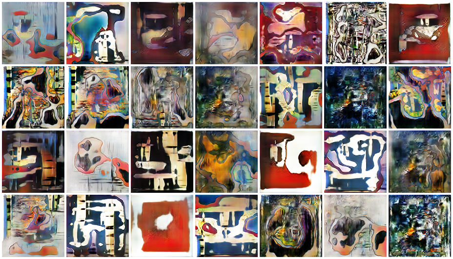
One of the most interesting ideas on the last decades in machine learning is the GAN architecture for generatine model. While GANs have shown remarkable success in generating high-quality images and other continuous data types, tabular data poses unique challenges. Tabular data often contains a mix of discrete and continuous variables, with complex dependencies between them. Traditional GAN architectures struggle to capture these intricacies, leading to poor performance when applied directly to tabular data. CTGAN addresses these challenges by introducing a specialized framework for generating realistic synthetic tabular data.
CTGAN Architecture #
The CTGAN model is based on the GAN framework, comprising two main components: a generator and a discriminator.
- Generator: The generator is responsible for producing synthetic data that resembles the real data. It takes as input a noise vector sampled from a standard normal distribution and a conditioning vector. The conditioning vector encodes specific values of categorical variables, enabling the generation of samples with particular characteristics. The generator outputs a vector representing a synthetic data sample, which includes both categorical and continuous features.
- Discriminator: The discriminator’s role is to distinguish between real and synthetic data samples. It is a binary classifier trained to maximize the likelihood of correctly identifying real data from the generator’s output. The discriminator receives both real and synthetic data as input and outputs a probability score indicating whether the input is real or fake.
Key Innovations in CTGAN #
CTGAN introduces several key innovations that enable it to handle the complexities of tabular data:
-
Conditional Vector and Mode-specific Normalization: This allows the generator to conditionally generate data based on specific categories. This is particularly useful in scenarios where some features are strongly dependent on others. For example, in a dataset with gender and age features, conditioning on gender can help the generator produce age values that are realistic for that gender. Mode-specific normalization is applied to continuous features during training, ensuring that each mode (category) is normalized independently. This prevents the generator from learning spurious correlations between categorical and continuous features.
-
Training by Sampling: To address the imbalance in categorical data, CTGAN uses a sampling strategy where the generator focuses on underrepresented categories during training. This ensures that the generator learns to produce realistic samples across all categories, not just the majority ones.
-
Logistic Loss for the Generator: The generator’s loss function is modified to include a logistic loss term. This encourages the generator to produce samples that are close to the decision boundary of the discriminator, promoting diversity in the generated samples. The inclusion of this term helps the generator avoid mode collapse, a common issue in GANs where the generator produces a limited variety of samples.
-
Training Process. The training process for CTGAN follows the standard GAN training procedure.
-
Preprocessing: The data is preprocessed to convert categorical variables into one-hot encoded vectors. Continuous variables are normalized using mode-specific normalization. The data is then split into real samples and conditional vectors.
The Math Behind GANs and CTGAN #
The description above is in words. In this section I want to write down the objectives that CTGAN actually optimizes. I start from the original GAN game, show why it amounts to minimizing a Jensen–Shannon divergence, explain why that motivates the Wasserstein loss with gradient penalty that CTGAN trains with, and then formalize CTGAN’s two tabular-specific ideas.
The minimax game and the optimal discriminator #
A generator $G$ maps noise $z \sim p_z$ to samples. Call the distribution of $G(z)$ $p_g$. A discriminator $D(x) \in (0, 1)$ outputs the probability that $x$ came from the data distribution $p_{\text{data}}$ and not from $G$. Goodfellow et al. define the game
$$\min_G \max_D\ V(D, G) = \mathbb{E}_{x \sim p_{\text{data}}}\big[\log D(x)\big] + \mathbb{E}_{z \sim p_z}\big[\log\big(1 - D(G(z))\big)\big].$$
For a fixed $G$, write the second expectation over $x \sim p_g$ and maximize pointwise. The integrand is $p_{\text{data}}(x)\log D(x) + p_g(x)\log(1 - D(x))$. The function $y \mapsto a\log y + b\log(1-y)$ has its maximum at $y = a/(a+b)$, so
$$D^*_G(x) = \frac{p_{\text{data}}(x)}{p_{\text{data}}(x) + p_g(x)}.$$
Substituting back and writing $m = \tfrac12(p_{\text{data}} + p_g)$ for the mixture, each log ratio picks up a $\log\tfrac12$:
$$\begin{aligned} V(D^*_G, G) &= \mathbb{E}_{p_{\text{data}}}\Big[\log\frac{p_{\text{data}}}{2m}\Big] + \mathbb{E}_{p_g}\Big[\log\frac{p_g}{2m}\Big] \\ &= -\log 4 + D_{\mathrm{KL}}(p_{\text{data}}\,\|\,m) + D_{\mathrm{KL}}(p_g\,\|\,m) \\ &= -\log 4 + 2\,\mathrm{JSD}(p_{\text{data}}\,\|\,p_g). \end{aligned}$$
So, with a perfect discriminator, training the generator minimizes the Jensen–Shannon divergence, and the global optimum is $p_g = p_{\text{data}}$ with $D^* \equiv \tfrac12$. In practice the generator maximizes $\mathbb{E}_z[\log D(G(z))]$ instead (the “non-saturating” loss), which has the same fixed point but stronger gradients early in training.
From JS to Wasserstein with gradient penalty #
The JS divergence has a well-known failure mode. When $p_{\text{data}}$ and $p_g$ have (nearly) disjoint supports, as is typical for distributions on low-dimensional manifolds, $\mathrm{JSD} = \log 2$ no matter how far apart they are. The discriminator saturates and the generator gets no useful gradient. WGAN replaces it with the Wasserstein-1 distance, written in its Kantorovich–Rubinstein dual form as a supremum over 1-Lipschitz critics $f$:
$$W(p_{\text{data}}, p_g) = \sup_{\|f\|_L \le 1}\ \mathbb{E}_{x \sim p_{\text{data}}}[f(x)] - \mathbb{E}_{\tilde x \sim p_g}[f(\tilde x)].$$
This keeps changing smoothly as $p_g$ moves, even with disjoint supports. A differentiable $f$ is 1-Lipschitz if and only if $\|\nabla f\| \le 1$ everywhere. Gulrajani et al. enforce this softly with a penalty on the critic’s gradient norm, measured at random points between real and fake samples. The critic $D$ (now an unbounded score, no sigmoid) minimizes
$$L_D = \mathbb{E}_{\tilde x \sim p_g}\big[D(\tilde x)\big] - \mathbb{E}_{x \sim p_{\text{data}}}\big[D(x)\big] + \lambda\, \mathbb{E}_{\hat x}\Big[\big(\|\nabla_{\hat x} D(\hat x)\|_2 - 1\big)^2\Big],$$
where $\hat x = \varepsilon x + (1-\varepsilon)\tilde x$ with $\varepsilon \sim \mathcal{U}[0,1]$ is a random point on the segment between a real sample $x$ and a fake one $\tilde x$. The default is $\lambda = 10$, and the generator minimizes $-\mathbb{E}_{z}[D(G(z))]$. This is the loss CTGAN trains with. Its critic also follows PacGAN, scoring packs of 10 samples jointly so that it can detect a lack of diversity, which helps against mode collapse.
Mode-specific normalization #
Here I use CTGAN’s notation. A table has continuous columns $C_1, \dots, C_{N_c}$ and discrete columns $D_1, \dots, D_{N_d}$, and $c_{i,j}$ is the value of column $C_i$ in row $j$. Continuous columns are often multimodal, so min-max scaling into $[-1, 1]$ for a $\tanh$ output works badly. Instead, each column $C_i$ is preprocessed in three steps.
- Fit a variational Gaussian mixture, which also picks the number of modes $m_i$: $\mathbb{P}_{C_i}(c_{i,j}) = \sum_{k=1}^{m_i} \mu_k\, \mathcal{N}(c_{i,j};\ \eta_k, \phi_k)$, where $\mu_k$, $\eta_k$, $\phi_k$ are the weight, mean and standard deviation of mode $k$.
- For each value, compute the mode densities $\rho_k = \mu_k\, \mathcal{N}(c_{i,j};\ \eta_k, \phi_k)$.
- Sample one mode $k$ with probability proportional to $\rho_k$. Encode the value as a one-hot mode indicator $\beta_{i,j}$ plus a scalar position within that mode:
$$\alpha_{i,j} = \frac{c_{i,j} - \eta_k}{4\phi_k}.$$
Because almost all of a Gaussian’s mass lies within $\pm 4\phi_k$ of its mean, $\alpha_{i,j}$ falls in $[-1, 1]$, which is exactly the range of a $\tanh$. With $d_{i,j}$ the one-hot encoding of discrete column $D_i$, a row becomes
$$r_j = \alpha_{1,j} \oplus \beta_{1,j} \oplus \dots \oplus \alpha_{N_c,j} \oplus \beta_{N_c,j} \oplus d_{1,j} \oplus \dots \oplus d_{N_d,j},$$
where $\oplus$ is concatenation. The generator outputs each $\alpha$ through a $\tanh$, and each $\beta$ and $d$ through a Gumbel-softmax.
The conditional generator and training-by-sampling #
Rare categories are the second problem. If rows are sampled uniformly, a category that appears in 1% of rows almost never shapes the generator’s gradients. CTGAN fixes this by conditioning. Pick a discrete column $D_{i^*}$ and a value $k^*$, and encode the condition $D_{i^*} = k^*$ with one mask vector $m_i$ per discrete column, of length $|D_i|$:
$$m_i^{(k)} = \begin{cases} 1 & \text{if } i = i^* \text{ and } k = k^*, \\ 0 & \text{otherwise,} \end{cases} \qquad \text{cond} = m_1 \oplus \dots \oplus m_{N_d}.$$
The generator receives $z \oplus \text{cond}$ and is meant to model $\mathbb{P}_G(\text{row} \mid D_{i^*} = k^*)$. Nothing in the architecture forces the generated one-hot $\hat d_{i^*}$ to agree with the condition. So the generator loss gets an extra term, the cross-entropy between $m_{i^*}$ and $\hat d_{i^*}$, averaged over the batch, on top of the WGAN term above.
Training-by-sampling decides which conditions to show:
- Choose the column $i^*$ uniformly among the $N_d$ discrete columns.
- Choose $k^*$ from a PMF over that column’s values in which each value’s mass is proportional to the logarithm of its frequency. Taking the log flattens the distribution, so minority categories are seen far more often than their frequency, but not uniformly.
- Build cond as above, and give the critic a real row that actually has $D_{i^*} = k^*$, so that it compares $\mathbb{P}_G(\text{row} \mid \text{cond})$ against $\mathbb{P}(\text{row} \mid \text{cond})$.
This resampling does not bias the model. If the generator learns every conditional correctly, $\mathbb{P}_G(\text{row} \mid D_{i^*} = k) = \mathbb{P}(\text{row} \mid D_{i^*} = k)$, then the true joint is recovered at generation time by drawing the condition from the real frequencies:
$$\mathbb{P}(\text{row}) = \sum_{k \in D_{i^*}} \mathbb{P}_G(\text{row} \mid D_{i^*} = k)\, \mathbb{P}(D_{i^*} = k).$$
Training uses the log-frequency distribution, so every category gets gradient signal. Sampling uses the true frequencies, so the synthetic table keeps the real marginals.
References #
- Ian J. Goodfellow, Jean Pouget-Abadie, Mehdi Mirza, Bing Xu, David Warde-Farley, Sherjil Ozair, Aaron Courville, Yoshua Bengio. Generative Adversarial Networks. NeurIPS 2014.
- Martin Arjovsky, Soumith Chintala, Léon Bottou. Wasserstein GAN. ICML 2017.
- Ishaan Gulrajani, Faruk Ahmed, Martin Arjovsky, Vincent Dumoulin, Aaron Courville. Improved Training of Wasserstein GANs. NeurIPS 2017.
- Lei Xu, Maria Skoularidou, Alfredo Cuesta-Infante, Kalyan Veeramachaneni. Modeling Tabular data using Conditional GAN. NeurIPS 2019.
Comments