Implementing the Kalman Filter in Python
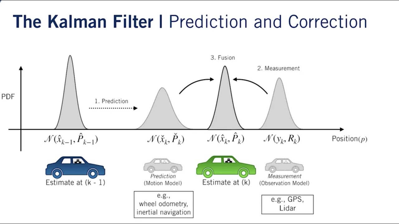
Hello. I’m trying to experiment with some recent articles that tries to connect transformers and kalman filter. I remember that I saw in my undergrad this concept on the control lecture but to be honest I didn’t quite understand the concept at the time. To help my understanding i tried to implement using only some basic python libraries the Kalman Filter in python.
Before the notebook with the implementation here is a quick summary of what is this filter provided by GPT ( =P ):
A Kalman filter is a powerful algorithm used for making estimates or predictions in systems that are subject to various uncertainties. It’s widely used in fields like robotics, aerospace, finance, and even weather forecasting. Here’s a simplified explanation suitable for a blog post:
-
Understanding the Kalman Filter: A Simple Guide Imagine you’re trying to predict the position of a moving car using a GPS system. The GPS provides you with location data, but this data isn’t perfect—it has some level of inaccuracy or ‘noise’. How do you make the best possible estimate of the car’s true position?
-
Enter the Kalman filter. Developed by Rudolf E. Kalman in the 1960s, this algorithm is a set of mathematical equations that provides an efficient computational (recursive) solution to the problem of estimating the state of a process—in our case, the position and speed of the car.
-
How Does It Work? The Kalman filter works in two fundamental steps: Prediction and Update.
-
Prediction: This step involves predicting the current state of the process (like the position and velocity of the car) based on the previous state. It’s like saying, “Given where the car was and how fast it was moving, here’s where I think it is now.”
-
Update: In this step, the Kalman filter takes new measurements (e.g., from the GPS) and refines the prediction. It essentially asks, “Now that I have new data, how should I adjust my prediction to be more accurate?”
The beauty of the Kalman filter lies in its ability to deal with uncertainty. It’s designed to weigh both the predicted state and the new measurements, considering the uncertainties in both. If the measurements are very accurate, it gives them more weight. If the predictions are believed to be more reliable, it leans more on them.
That weighing is the Kalman gain, and it is worth playing with directly. Below,
a hidden state does a random walk and you only ever see the noisy dots. The two
sliders do not change the data — they change what the filter believes about
the noise. Push Q down and it decides the state can barely move, so it
smooths hard and lags; push Q up and it chases every measurement. In between
it beats the raw sensor by a wide margin.
One thing worth noticing: only the ratio Q/R affects the estimate. Scale
both up by a thousand and the red line does not move at all — but the
uncertainty band does, because the filter now believes it is far less sure than
it really is.
The equations behind the sliders #
The summary above is the intuition. Here is the derivation I didn’t follow back in undergrad. It turns out to be short once you see that the whole filter is just Gaussian conditioning, repeated.
The linear-Gaussian state space model #
The hidden state at time $t$ is $x_t \in \mathbb{R}^n$ and the measurement is $y_t \in \mathbb{R}^m$. The model is
$$x_t = A x_{t-1} + w_t, \qquad w_t \sim \mathcal{N}(0, Q),$$
$$y_t = H x_t + v_t, \qquad v_t \sim \mathcal{N}(0, R),$$
with initial state $x_0 \sim \mathcal{N}(m_0, P_0)$. Here $A \in \mathbb{R}^{n\times n}$ is the transition (dynamics) matrix, $H \in \mathbb{R}^{m \times n}$ maps a state to what the sensor would read, and $Q$ and $R$ are the process and measurement noise covariances. The noises $w_t$, $v_t$ and $x_0$ are mutually independent. For the car, $x_t$ could be (position, velocity), $A$ could be constant-velocity kinematics, and $H = (1\;\, 0)$ because the GPS reports only position.
The goal is the filtering distribution $p(x_t \mid y_{1:t})$. Everything in the model is linear and Gaussian, so this distribution stays Gaussian, $\mathcal{N}(m_t, P_t)$. We only need to track a mean $m_t$ and a covariance $P_t$.
Predict #
Push the previous belief $\mathcal{N}(m_{t-1}, P_{t-1})$ through the dynamics. A linear map of a Gaussian plus independent Gaussian noise is Gaussian, with
$$m_t^- = A\, m_{t-1}, \qquad P_t^- = A P_{t-1} A^\top + Q .$$
This is $p(x_t \mid y_{1:t-1}) = \mathcal{N}(m_t^-, P_t^-)$, the “here’s where I think the car is now” step. The dynamics carry the old uncertainty forward through $A$, and $Q$ adds fresh uncertainty on top.
Update #
When $y_t$ arrives:
$$\begin{aligned} \tilde{y}_t &= y_t - H m_t^- && \text{(innovation)} \\ S_t &= H P_t^- H^\top + R && \text{(innovation covariance)} \\ K_t &= P_t^- H^\top S_t^{-1} && \text{(Kalman gain)} \\ m_t &= m_t^- + K_t \tilde{y}_t \\ P_t &= (I - K_t H) P_t^- . \end{aligned}$$
Why the update looks like this: conditioning a joint Gaussian #
Given $y_{1:t-1}$, the pair $(x_t, y_t)$ is jointly Gaussian because $y_t = H x_t + v_t$ is linear in $x_t$ with independent noise. Its mean and covariance are
$$\begin{pmatrix} x_t \\ y_t \end{pmatrix} \Big|\, y_{1:t-1} \sim \mathcal{N}\!\left( \begin{pmatrix} m_t^- \\ H m_t^- \end{pmatrix}, \begin{pmatrix} P_t^- & P_t^- H^\top \\ H P_t^- & H P_t^- H^\top + R \end{pmatrix} \right).$$
The standard result for conditioning a Gaussian is: if $(a, b)$ is jointly Gaussian with means $\mu_a, \mu_b$ and covariance blocks $\Sigma_{aa}, \Sigma_{ab}, \Sigma_{ba}, \Sigma_{bb}$, then
$$a \mid b \sim \mathcal{N}\big(\mu_a + \Sigma_{ab}\Sigma_{bb}^{-1}(b - \mu_b),\; \Sigma_{aa} - \Sigma_{ab}\Sigma_{bb}^{-1}\Sigma_{ba}\big).$$
Substitute $a = x_t$, $b = y_t$. Then $\Sigma_{ab}\Sigma_{bb}^{-1} = P_t^- H^\top S_t^{-1} = K_t$, and we get
$$m_t = m_t^- + K_t (y_t - H m_t^-), \qquad P_t = P_t^- - K_t H P_t^- = (I - K_t H) P_t^- .$$
That is the whole update. The Kalman gain is the regression coefficient of the state on the measurement under the predicted distribution.
The same answer can be read as an MMSE estimate. For jointly Gaussian variables the conditional mean $\mathbb{E}[x_t \mid y_{1:t}]$ minimises the expected squared error over all estimators. Among estimators of the form $m_t^- + K\tilde{y}_t$, it is also the choice of $K$ that minimises $\operatorname{tr} P_t$. The error covariance of such an estimator is $(I-KH)P_t^-(I-KH)^\top + K R K^\top$. Differentiate its trace with respect to $K$ and set the result to zero: $-2 P_t^- H^\top + 2 K S_t = 0$, which gives $K = P_t^- H^\top S_t^{-1} = K_t$.
The scalar case: a product of two Gaussians #
For the widget’s local-level model, $A = H = 1$ and every quantity is a scalar. Then the update is Bayes’ rule with a Gaussian prior $\mathcal{N}(m_t^-, P_t^-)$ and a Gaussian likelihood $\mathcal{N}(y_t;\, x_t, R)$. Their product is a Gaussian whose precisions add and whose mean is a precision-weighted average:
$$\frac{1}{P_t} = \frac{1}{P_t^-} + \frac{1}{R}, \qquad m_t = \frac{R\, m_t^- + P_t^-\, y_t}{P_t^- + R} = m_t^- + K_t (y_t - m_t^-), \qquad K_t = \frac{P_t^-}{P_t^- + R} \in (0, 1).$$
This is the “weigh both” sentence above, made exact. A precise sensor ($R \to 0$) gives $K_t \to 1$, so the filter follows the measurement. A confident prediction ($P_t^- \to 0$) gives $K_t \to 0$, so it ignores the measurement.
It also explains the ratio remark from the widget. Divide every variance by $R$ and write $p = P/R$ and $q = Q/R$. The recursion becomes $p_t^- = p_{t-1} + q$, $K_t = p_t^-/(p_t^- + 1)$, $p_t = (1 - K_t)\, p_t^-$. So the gains, and therefore the red line, depend only on $Q/R$ (and on $P_0/R$, whose effect washes out after a few steps). The absolute variance $P_t = R\, p_t$ still scales with $R$, which is why the band moves.
- Real-World Applications While the GPS example is straightforward, the Kalman filter is used in much more complex situations. It’s vital in the operation of satellites and spacecraft, where precise navigation is crucial. In the financial world, it helps in predicting market trends and in robotics, it’s used for navigation and tracking movements.

Finally here is the notebook : Colab
References #
-
-
- Kalman (1960). A New Approach to Linear Filtering and Prediction Problems. Journal of Basic Engineering 82(1), 35–45.
-
-
- Welch, G. Bishop (1995). An Introduction to the Kalman Filter. Technical Report TR 95-041, University of North Carolina at Chapel Hill.
-
- Särkkä (2013). Bayesian Filtering and Smoothing. Cambridge University Press.
Comments