Hopfield Networks for dummies
Introduction to Hopfield Networks #
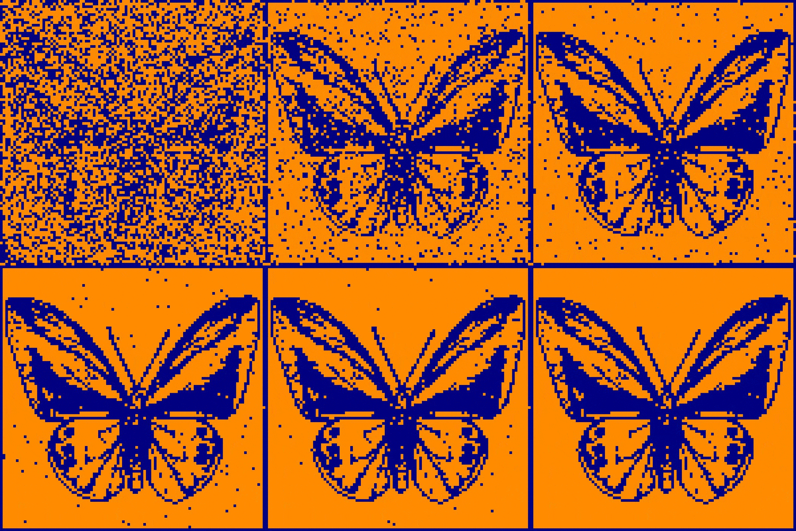
Hopfield Networks, a type of Recurrent Neural Network (RNN), are renowned for their unique ability to store and retrieve patterns through associative memory. This means they can recall a complete memory from just a partial input. Inspired by the Ising model in physics, which explains magnetic behaviors in certain materials, Hopfield Networks use a system of interconnected neurons, each able to be in one of two states, akin to magnetic dipoles. These neurons are fully connected, each influencing the other based on the strength of their connections. The network dynamically evolves to a stable state where the system’s ‘energy’ is minimized, representing a memory. The overall network state thus can represent binary information, like an image or a pattern, making Hopfield Networks particularly effective in pattern recognition and completion tasks.
That last sentence is much easier to believe once you have watched it happen, so here is a real one — 144 neurons, three stored patterns, Hebbian weights, and the asynchronous update rule running in your browser. Draw on the grid, corrupt a memory, and press Recall.
The classical network, formally #
Before going modern, I want to write down the three facts that make the widget above work: the energy, the reason it can only go down, and where the weights come from.
State, weights and energy #
The network has $N$ neurons with states $s_i \in \{-1, +1\}$, collected in a vector $s \in \{-1,+1\}^N$. The weights form a matrix $W \in \mathbb{R}^{N \times N}$ that is symmetric ($w_{ij} = w_{ji}$) with zero diagonal ($w_{ii} = 0$), and each neuron has a threshold $\theta_i$. The energy of a state is
$$E(s) = -\frac{1}{2} s^\top W s + \theta^\top s = -\frac{1}{2}\sum_{i \neq j} w_{ij} s_i s_j + \sum_i \theta_i s_i .$$
This is exactly the Ising energy with couplings $w_{ij}$ and external field $-\theta_i$, which is the physics connection from the introduction.
Asynchronous updates never increase the energy #
Define the local field of neuron $i$ as $h_i = \sum_{j} w_{ij} s_j - \theta_i$. The asynchronous rule picks one neuron $i$ at a time and sets
$$s_i' = \operatorname{sgn}(h_i),$$
leaving $s_i$ unchanged when $h_i = 0$. Only the terms of $E$ that contain $s_i$ can change. Using symmetry and $w_{ii} = 0$, those terms are $-s_i \sum_{j \neq i} w_{ij} s_j + \theta_i s_i = -s_i h_i$ (the factor $\tfrac{1}{2}$ disappears because $s_i$ shows up once as $s_i s_j$ and once as $s_j s_i$). So flipping $s_i$ to $s_i'$ changes the energy by
$$\Delta E = -(s_i' - s_i)\, h_i .$$
There are two cases. If $s_i' = s_i$ then $\Delta E = 0$. Otherwise $s_i' - s_i = 2 s_i' = 2\operatorname{sgn}(h_i)$, and
$$\Delta E = -2\operatorname{sgn}(h_i)\, h_i = -2|h_i| < 0 .$$
So every update leaves $E$ unchanged or strictly lowers it. Since there are only $2^N$ states, $E$ is bounded below and the dynamics must stop at a state where no single flip lowers the energy, a local minimum. That is why $E$ is a Lyapunov function. Both assumptions are needed. With asymmetric weights the argument breaks and the network can cycle. With synchronous updates (all neurons at once) it can oscillate between two states.
The Hebbian rule #
To store $P$ patterns $\xi^1, \dots, \xi^P \in \{-1,+1\}^N$ we use Hebb’s “fire together, wire together”:
$$w_{ij} = \frac{1}{N} \sum_{\mu=1}^{P} \xi^\mu_i \xi^\mu_j \quad (i \neq j), \qquad w_{ii} = 0 .$$
In matrix form this is $W = \frac{1}{N}\sum_\mu \xi^\mu (\xi^\mu)^\top - \frac{P}{N} I$. With $\theta = 0$, ask whether a stored pattern $\xi^\nu$ is a fixed point. Its local field is
$$h_i = \frac{1}{N}\sum_{j \neq i}\sum_{\mu} \xi^\mu_i \xi^\mu_j \xi^\nu_j = \underbrace{\frac{N-1}{N}\,\xi^\nu_i}_{\text{signal}} + \underbrace{\frac{1}{N}\sum_{\mu \neq \nu}\sum_{j \neq i} \xi^\mu_i \xi^\mu_j \xi^\nu_j}_{\text{crosstalk } C^\nu_i} .$$
The signal term points the right way. The crosstalk term is what the other memories contribute.
Capacity: about 0.138 N #
For random patterns, the crosstalk $C^\nu_i$ is a sum of about $(P-1)(N-1)$ independent $\pm 1$ terms divided by $N$. By the central limit theorem it is roughly Gaussian with mean $0$ and variance $\approx P/N$. Bit $i$ of $\xi^\nu$ is unstable when the crosstalk beats the signal, i.e. when $\xi^\nu_i C^\nu_i < -1$, which happens with probability about
$$P_{\text{error}} \approx \Phi\!\left(-\sqrt{N/P}\right),$$
where $\Phi$ is the standard normal CDF. So what matters is the load $\alpha = P/N$. As $\alpha$ grows, the noise standard deviation $\sqrt{\alpha}$ approaches the signal, and the stored patterns stop being minima.
This one-step picture ignores something: an early flip changes the field seen by the other neurons, and errors can snowball. The exact answer comes from a statistical-mechanics (replica) analysis by Amit, Gutfreund and Sompolinsky. I’ll state it as a result. In the limit $N \to \infty$, retrieval states close to the stored patterns exist only for
$$\alpha = \frac{P}{N} < \alpha_c \approx 0.138 .$$
Even below that, the retrieved state has a small fraction of wrong bits. Above $\alpha_c$ the memory collapses into spurious “spin-glass” states. So a classical network with 144 neurons, like the one in the widget, can hold only about 20 random patterns. That linear scaling is the limitation the modern version removes.
Hopfield Networks is all you need #
Now with a little bit of more context of Hopfield Networks’s we will dive into a quick summary of the Paper. To put it simply the main message of the paper is the following: By introducing a modern Hopfield Network with continuous states we can store exponentially many patterns, retrieve them with only one update and the update rule is equivalent to the attention mechanism used in transformers.
Now let’s dive little deep into the details. The basic architecture is on

The evolution of Hopfield Networks towards modern architectures involves a transition from binary to continuous neuron states, allowing for more complex and nuanced representations. This advancement closely aligns with the mechanisms used in transformer models in deep learning. The modern approach introduces a new energy function to accommodate these continuous states, fundamentally changing the network dynamics. The update rule in these modern networks parallels the attention mechanism in transformer and BERT models, marking a significant innovation. Modern Hopfield Networks not only enhance the capacity for pattern storage and retrieval but also exhibit improved efficiency in these processes. The research also presents several theorems to explain the behavior of these networks, including their convergence, storage capacity, pattern retrieval efficiency, and error rates. These networks extend beyond mimicking transformer attention, offering potential applications in a wide range of deep learning architectures and providing new tools for designing advanced neural network systems.
The paper introduces 5 theorems to characterize the introduced hopfield network.
-
Theorem 1: It states that the update rule for these networks converges globally. This means for a given sequence of states, the energy will eventually converge to a stable value at a fixed point, even as time tends to infinity. The proof involves the Concave-Convex Procedure (CCCP) to ensure this global convergence.
-
Theorem 2: This theorem extends Theorem 1, stating that not only does the energy converge, but the sequence of states either converges or its limit points form a connected and compact set of stationary points. If this set is finite, the sequence will converge to a specific stationary point.
-
Theorem 3: This theorem discusses the storage capacity of the network. It defines conditions under which a certain number of random patterns can be stored with a high probability. The calculations involve complex functions like the Lambert W function and take into account the dimensions of the pattern space and a failure probability.
-
Theorem 4: It states that the network is capable of retrieving patterns efficiently with just one update, particularly if the patterns are well-separated. The theorem quantifies the retrieval capability in terms of the separation of patterns.
-
Theorem 5: This theorem addresses the retrieval error, which is found to be exponentially small relative to the pattern separation. It provides bounds on this error, demonstrating the effectiveness of the network in accurately retrieving patterns.
The modern energy, and why its update is attention #
The bullet points above are easier to understand once the equations are written out, so here they are. Store $N$ continuous patterns $x_1, \dots, x_N \in \mathbb{R}^d$ as the columns of $X = (x_1, \dots, x_N) \in \mathbb{R}^{d \times N}$, and let the state (the query) be $\xi \in \mathbb{R}^d$. For an inverse temperature $\beta > 0$, define the log-sum-exp
$$\operatorname{lse}(\beta, z) = \beta^{-1} \log \sum_{l=1}^{N} \exp(\beta z_l), \qquad z \in \mathbb{R}^N ,$$
which is a smooth maximum: as $\beta \to \infty$ it tends to $\max_l z_l$. The energy of Ramsauer et al. is
$$E(\xi) = -\operatorname{lse}(\beta, X^\top \xi) + \frac{1}{2}\xi^\top \xi + \beta^{-1}\log N + \frac{1}{2} M^2 ,$$
where $M = \max_i \lVert x_i \rVert$. The last two terms are constants that keep $E$ bounded and non-negative. The first term rewards a state that has a large dot product with some stored pattern. The second term keeps $\xi$ from running off to infinity.
Deriving the update. $E$ is a convex function minus a convex function: $\frac{1}{2}\xi^\top\xi$ is convex, and so is $\operatorname{lse}$ composed with the linear map $\xi \mapsto X^\top\xi$. The Concave-Convex Procedure (CCCP) minimises such a difference by linearising the concave part, $-\operatorname{lse}$, at the current point and minimising the convex surrogate that results. Setting the gradient of the surrogate to zero gives
$$\nabla_\xi \Big(\tfrac{1}{2}\xi^\top\xi\Big)\Big|_{\xi^{\text{new}}} = \nabla_\xi \operatorname{lse}(\beta, X^\top\xi)\Big|_{\xi} .$$
The left side is just $\xi^{\text{new}}$. For the right side, the gradient of $\operatorname{lse}(\beta, z)$ with respect to $z$ is $\operatorname{softmax}(\beta z)$, and the chain rule through $z = X^\top \xi$ multiplies by $X$. So
$$\xi^{\text{new}} = X \operatorname{softmax}(\beta X^\top \xi) .$$
CCCP guarantees $E(\xi^{\text{new}}) \le E(\xi)$, the continuous version of the monotonicity proof above. This is the starting point for Theorems 1 and 2.
Why this is attention. Read the update literally. It scores the query against every stored pattern with a dot product ($X^\top\xi$), turns the scores into weights with a softmax, and returns the weighted average of the stored patterns. Now stack several queries as rows. Let the queries be projections of inputs $R$, $Q = R W_Q$, and the stored patterns be projections of $Y$, $K = Y W_K$. Set $\beta = 1/\sqrt{d_k}$, apply the update to every query at once (softmax row-wise), and project the result with $W_V$. The result is
$$Z = \operatorname{softmax}\!\left(\frac{1}{\sqrt{d_k}} Q K^\top\right) V, \qquad V = K W_V ,$$
which is transformer attention. One attention layer is therefore one step of energy descent on a modern Hopfield network. The paper’s capacity results say the number of patterns that can be stored grows exponentially in $d$, and a well-separated pattern is retrieved after this single step. The temperature also explains the fixed points listed below. With small $\beta$ the softmax is nearly uniform and $\xi^{\text{new}}$ lands near the mean of the patterns (the global fixed point). With large $\beta$ it is nearly one-hot and recovers a single pattern. In between, it averages over a cluster of similar patterns (a metastable state).
Finally it is interesting to note the following.
-
In modern Hopfield networks, the dynamics of pattern convergence are
characterized by:
-
If patterns xi are not well separated, the iteration converges to a global fixed point near the average of all vectors.
-
In cases where some patterns are similar yet distinct from others, a metastable state near these patterns is formed. Iterations converge to this metastable state.
-
-
Hopfield Update Rule as Transformer Attention
-
The Hopfield network update rule parallels the attention mechanism in transformer and BERT models.
-
With stored (key) patterns yi and state (query) patterns ri, and using transformations with weight matrices WK, WQ, and WV, the update rule resembles transformer attention.
-
The equivalence is shown in the formulation of transformer self-attention, where modifications in weight matrices and softmax function applications are highlighted.
-
- Applications in Deep Network Architectures Hopfield networks extend beyond the attention mechanism, offering additional functionalities in deep learning architectures through specific layers.
Checking it numerically #
Here is the monotonicity proof and the one-step retrieval claim tested in a few lines of NumPy. The first half stores five patterns with the Hebbian rule, corrupts one, and records the energy after every single asynchronous update. The second half runs one modern-Hopfield update on 1000 stored patterns.
import numpy as np

rng = np.random.default_rng(0)
N, P = 100, 5                                  # neurons, stored patterns

# Hebbian weights with zero diagonal
patterns = rng.choice([-1, 1], size=(P, N))
W = patterns.T @ patterns / N
np.fill_diagonal(W, 0.0)
theta = np.zeros(N)                            # thresholds

def energy(s):
    return -0.5 * s @ W @ s + theta @ s

# corrupt pattern 0 by flipping 30% of its bits
s = patterns[0].copy()
flip = rng.choice(N, size=30, replace=False)
s[flip] *= -1

energies = [energy(s)]
for sweep in range(5):
    for i in rng.permutation(N):               # asynchronous updates
        h = W[i] @ s - theta[i]
        if h != 0:
            s[i] = 1 if h > 0 else -1
        energies.append(energy(s))

steps = np.diff(energies)
print("energy: start %.3f, end %.3f" % (energies[0], energies[-1]))
print("largest single-step change: %.2e (never positive)" % steps.max())
print("overlap with stored pattern:", int(s @ patterns[0]), "/", N)

# Modern Hopfield: one update xi_new = X softmax(beta X^T xi) is attention
d, M = 64, 1000                                # dimension, stored patterns
X = rng.standard_normal((d, M))                # stored patterns as columns
target = 123
xi = X[:, target] + 0.5 * rng.standard_normal(d)   # noisy query

def softmax(z):
    z = z - z.max()
    e = np.exp(z)
    return e / e.sum()

beta = 1.0
xi_new = X @ softmax(beta * X.T @ xi)
best = np.argmax(X.T @ xi_new)
err = np.linalg.norm(xi_new - X[:, target]) / np.linalg.norm(X[:, target])
print("one-step retrieval picks pattern", best, "(target %d), relative error %.1e" % (target, err))References #
-
-
- Hopfield (1982). Neural networks and physical systems with emergent collective computational abilities. PNAS 79(8), 2554–2558.
-
-
-
- Amit, H. Gutfreund, H. Sompolinsky (1985). Storing infinite numbers of patterns in a spin-glass model of neural networks. Physical Review Letters 55, 1530.
-
-
- Hertz, A. Krogh, R. G. Palmer (1991). Introduction to the Theory of Neural Computation. Addison-Wesley.
-
- Krotov, J. J. Hopfield (2016). Dense Associative Memory for Pattern Recognition. NeurIPS. arXiv:1606.01164
-
- Demircigil, J. Heusel, M. Löwe, S. Upgang, F. Vermet (2017). On a model of associative memory with huge storage capacity. J. Stat. Phys. 168, 288–299. arXiv:1702.01929
-
- Ramsauer et al. (2020). Hopfield Networks is All You Need. arXiv:2008.02217
Comments